Journal of Water Resource and Protection
Vol. 3 No. 1 (2011) , Article ID: 3781 , 9 pages DOI:10.4236/jwarp.2011.31009
Analytical Solution to the One-Dimensional Advection-Diffusion Equation with Temporally Dependent Coefficients
Department of Mathematics and Astronomy, Lucknow University, Lucknow, India
E-mail: dilip3jais@gmail.com, atul.tusaar@gmail.com, yadav_rr2@yahoo.co.in
Received October 8, 2010; revised November 20, 2010; accepted December 23, 2010
Keywords: Advection, Diffusion, Dispersion, Continuous Input, Flux Type Condition
ABSTRACT
In a one-dimensional advection-diffusion equation with temporally dependent coefficients three cases may arise: solute dispersion parameter is time dependent while the flow domain transporting the solutes is uniform, the former is uniform and the latter is time dependent and lastly the both parameters are time dependent. In the present work analytical solutions are obtained for the last case, studying the dispersion of continuous input point sources of uniform and increasing nature in an initially solute free semi-infinite domain. The solutions for the first two cases and for uniform dispersion along uniform flow are derived as particular cases. The dispersion parameter is not proportional to the velocity of the flow. The Laplace transformation technique is used. New space and time variables are introduced to get the solutions. The solutions in all possible combinations of increasing/decreasing temporal dependence are compared with each other with the help of graphs. It has been observed that the concentration attenuation with position and time is the fastest in case of decreasing dispersion in accelerating flow field.
1. Introduction
Immiscible solute or tracer particles of pollutants are major cause of degradation of the hydro-environment in the surface water bodies and aquifers. The sources of such pollutants originate from human activities on the earth. Solute particles reach a surface water body with waste water drainage and reach an aquifer due to infiltrations from wastes disposal sites, underground septic tanks, mines and polluted water bodies that recharge the aquifers. Solutes are transported down the stream along the flow and disperse due to combined effects of diffusion and advection. Concentration attenuation with position and time is described by an advection-diffusion equation which is a partial differential equation of parabolic type. Due to growing concern about the safe hydro-environment for the existence of life on the earth the advection-diffusion equation has drawn significant attention of environmentalists, hydrologists, civil engineers and mathematical modelers. Its analytical and numerical solutions for the set of initial condition and boundary conditions typical for real situations are useful to assess the time and position at which the concentration level of the pollutants will start affecting the health of the habitats in the polluted water eco-system. Also such solutions help estimate and examine the rehabilitation process and management of a polluted water body after elimination of the pollution.
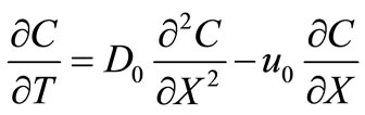
In the earlier analytical solutions the solute dispersion parameter and velocity have been considered constant in a homogeneous medium. The basic approach was to reduce the advection-diffusion equation
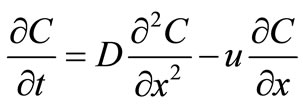 (1)
(1)
into a diffusion equation by eliminating the advection term. It was done either by introducing moving coordinates
 ,
,  (2)
(2)
or by introducing another dependent variable
 (3)
(3)
For example the analytical solution of the advectiondiffusion equation with constant coefficients in an initially solute free semi-infinite domain for a continuous uniform input point source  at the origin has been reported by Ogata and Banks [1], Harleman and Rumer [2], Guvanasen and Volker [3], Marshall et al. [4], by using the transformations in Equation (2), as
 (4)
(4)
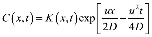
or by using the transformation in Equation (3), as
 (5)
(5)
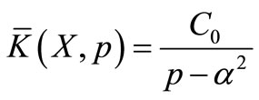
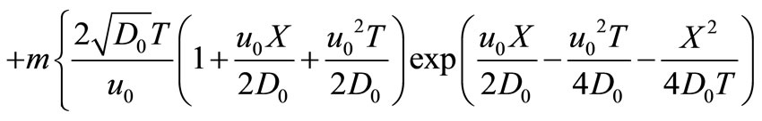
by Banks and Ali [5], Ogata [6], Lai and Jurinak [7], Marino [8] and Al-Niami and Rushton [9]. Both the solutions have been obtained by using Laplace transformation technique. The former solution satisfies the advection-diffusion equation but does not satisfy the input condition. The omission of factor  in Equation (4) makes the difference between the value of
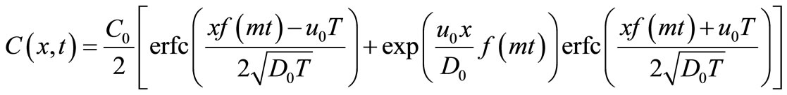
  at
at  obtained from this solution and that given by the input source condition, just half. Also this difference decreases for a smaller value of the velocity. The latter solution satisfies the input source condition and does not satisfy the differential equation but the error of approximation is of negligible order. So the latter type of analytical solutions have been obtained for different dispersion problems incorporating the other factors such as zero order production, first order decay, adsorption. Such solutions are compiled by van Genuchten and Alves [10] and Lindstrom and Boersma [11]. Such solutions are very useful in validating the numerical solutions.
Previous investigations have established that the longitudinal dispersion coefficient was directly proportional to Darcy velocity for a broad range of Reynold’s number. Taking advantage of this relationship, analytical solutions were obtained for a class of unsteady flow problems (Jaiswal et al., [12], Kumar et al., [13]). Further Yates [14] considered an exponentially decreasing dispersion along a uniform flow through porous medium to solve the advection-diffusion equation without adsorption. Logan and Zlotnik [15] and Logan [16] extended the works of Yates by including the adsorption and decay effects and studying their interactions with the heterogeneity caused by scale-dependent dispersion of periodic input source along uniform flow. Aral and Liao [17] obtained analytical solutions to two dimensional advection-dispersion equation with time dependent dispersion coefficients by eliminating convective terms by introducing moving coordinate systems and using superposition method (Haberman, [18]). Such assumptions were based on the observations of Matheron and De Marsily [19], Sposito et al. [20], Gehler et al. [21] who showed that large subsurface formations exhibit variable dispersivity properties, either as a function of distance or as a function of time along uniform flow. But such dependency may be more prevalent in surface water bodies due to local effects like curved boundaries, bridges etc., and chemically reactive type of pollutants whose dispersion may marginally increase or decrease with time. To understand the hydro-environment degradation problem in wider perspective, while investigating unsteady dispersion problems, all the three cases 1) unsteady dispersion along uniform flow, 2) uniform dispersion along unsteady flow and 3) unsteady dispersion along unsteady velocity but both being not proportional to each other, should be investigated. In a recent paper Jaiswal et al. [12] studied the first case and obtained the analytical solutions for pulse type uniform and varying inputs.
The present paper considers the general case 3) and analytical solutions similar to those in Equation (5) are derived by reducing the time dependent coefficients of the advection-diffusion equation into constant coefficients with the help of a set of new independent variables of space and time different from those in the earlier work and then using Laplace transformation technique. Continuous input point sources of uniform and increasing nature are considered. The analytical solutions for the first two cases and that of uniform dispersion along uniform flow may be obtained from this solution as particular cases. The solutions in different cases are illustrated and compared with each other.
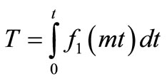
2. Temporally Dependent Dispersion along Unsteady Flow
The general linear form of one-dimensional advectiondiffusion equation in Cartesian system is
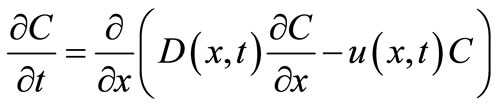 (6)
(6)
The symbol,  is the solute concentration at position
  of the domain at time
 . If the two coefficients
  and
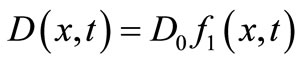
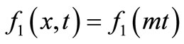
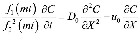
and  are constants then they are referred to as solute dispersion coefficient and uniform velocity, respectively, and the above equation reduces to Equation (1). Let us write the solute dispersion parameter and the velocity of the flow in the above advection-diffusion equation as
 and
and  (7)
(7)
In the present study it is assumed that the solute dispersion and the velocity of the flow, both are temporally dependent hence we consider
 and
and  (8)
(8)
where  is a resistive of dimension being inverse of time variable. Thus
  and
and  are non-dimensional expressions. It is chosen such that
  and
and  when either
  (represents the case of uniform dispersion along uniform flow) or
  (the initial stage). The advection-diffusion equation in Equation (6) assumes the form
 (9)
(9)
We study the dispersion of a continuous input point source introduced at the origin of an initially solute free one-dimensional semi-infinite medium. Analytical solutions are obtained for uniform input point source and that of increasing nature.
2.1. Uniform Input Point Source
In case of uniform continuous input point source the initial and boundary conditions for the above advectiondiffusion equation are
 ;
; ,
,  , (10)
 ;
; ,
,  , (11)
 ;
; ,
, (12)
(12)
Let us introduce a new space variable , using a transformation which is
 (13)
(13)
in terms of which the advection-diffusion equation in Equation (9) reduces to
 (14)
(14)
Further a new variable,  is introduced by the transformation
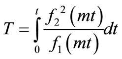 (15)
(15)
It is evident that the dimension of it will be that of time variable  hence it is referred to as a new time variable. While choosing expressions for
  and
and  it is also ascertained that
  at
at . So the nature of the initial condition does not change in the new time domain. The advection-diffusion equation in Equation (14) reduces to one with constant coefficients which is
 (16)
(16)
The conditions in Equations (10) - (12) may be written in terms of new independent variables as
 ;
; ,
, (17)
(17)
 ;
; ,
,  (18)
(18)
 ;
; ,
,  (19)
(19)
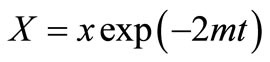
Now advection-diffusion equation in  domain given by Equation (16) is reduced into a diffusion equation in terms of a new independent variable,
  defined by
 (20)
(20)
which is
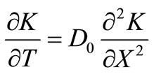 (21)
(21)
The conditions in Equations (17) - (19) reduce to
 ;
; ,
,  (22)
(22)
 ;
; ,
,  ,
,
where  (23)
(23)
 ;
; ,
,  (24)
(24)
respectively. Applying Laplace transformation above initial and boundary value problem reduces to an ordinary second order boundary value problem, which comprises of following three equations
 ;
;  (25)
(25)
 ;
;  (26)
(26)
 ;
;  (27)
(27)
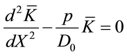
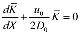
The particular solution of this boundary value problem may be obtained as
 (28)
(28)
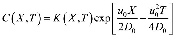
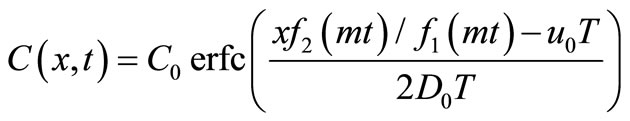
Applying inverse Laplace transformation on it, using the appropriate tables (van Genuchten and Alves, [10]) and using the necessary transformations defined earlier in the text, backwards, we may get the desired analytical solution as
 (29)
(29)
where  is defined in Equation (15). Also an analytical solution of the same initial and boundary value problem similar to that in Equation (4) may be obtained as either
 ;
;
 (30)
(30)
or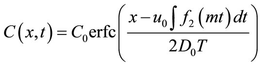 ;
;
 (31)
(31)
where (1/2) is omitted because of the reason stated below the solution in Equation (4).
2.2. Input Point Source of Increasing Nature
Due to increasing human activities the input point source may not remain constant instead it will increase with time. This premise is expressed by a mixed type nonhomogeneous condition as
 ;
; ,
, (32)
(32)
Using the expressions in Equation (6) it may be written in terms of and new independent variables defined in Equations (13) and (15), respectively, as
 ;
; ,
,  (33)
(33)
To proceed with it expressions  and
and  are considered. For these expressions the new space variable and new time variable will be given by
 (34)
(34)
 (35)
(35)
Solving old time variable  in terms of new time variable
  from the expression in Equation (35), and using that relationship, the condition in Equation (33) may be written as
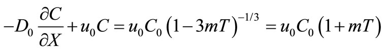 ;
;
 ,
,  (36)
(36)
where the series  is neglected from the binomial expansion as
  is chosen much smaller than one. Using the transformation in Equation (20), above condition may be written as
 ;
;
 ,
, (37)
(37)
Applying Laplace transformation on it we may get
 ;
;
 (38)
(38)
The particular solution of the boundary value problem comprising of Equations (25), (38) and (27) may be obtained as
 (39)
(39)
Applying inverse Laplace transformation on it, using the appropriate tables (van Genuchten and Alves, [10]) and using the necessary transformations defined in the text, backwards, we may get the desired analytical solution as

 (40)
(40)
where  and
and  are given by Equations (34) and (35), respectively.
2.3. Particular Cases
2.3.1. Uniform Dispersion along Unsteady Flow
An analytical solution of the dispersion problem in which solutes of a uniform input point source disperse uniformly along a flow domain of temporally dependent velocity under the same conditions may be obtained by substituting
 and
and  (41)
(41)
the solution in Equation (29) as
 (42)
(42)
The new time variable in this solution has the expression
 (43)
(43)
Similarly the analytical solution of this particular problem in case of increasing input point source will be defined by the solution (40) but the expressions for the new space and time variables will be
 and
and 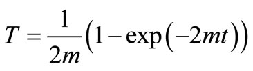 (44)
(44)
2.3.2. Temporally Dependent Dispersion along Uniform Flow
The analytical solutions of this particular dispersion problem in case of uniform and increasing input point sources may be obtained by substituting
 and
and  (45)
(45)
in the solutions in Equation (29) and Equation (40) which have been obtained independently in a recent work (Jaiswal et al., [12]).
2.3.3. Uniform Dispersion along Uniform Flow
The analytical solutions in this particular dispersion problem may be obtained by substituting
 and
and  (46)
(46)
in the solutions in Equation (29) and Equation (40), which are reported as problems (A1) and (A2), respectively, in time domain , by van Genuchten and Alves [10].
3. Result and Discussions
The solution in Equation (29) describes the solute dispersion of uniform input point source concentration through a medium in all the four cases of temporal dependence of the two coefficients of the advection-diffusion equation: 1) temporally dependent solute dispersion along temporally dependent flow, 2) temporally dependent dispersion along uniform flow, 3) uniform dispersion along temporally dependent flow and 4) uniform dispersion along uniform flow. The analytical solutions for last three cases may be obtained from (29) for ,
, ;
; ,
,  and
and ,
,  , respectively. The concentration values
  are evaluated from the solution in Equation (29) in all the above four cases and are illustrated in Figures (1)-(4). Temporal dependences of increasing and decreasing nature are considered. The different combinations for which the curves in these figures are drawn are given in table 1. The last combination may be obtained by putting
  in any of the first six combinations. Concentration values are evaluated in a long domain
  at
at . The values assigned to different parameters to draw these four figures are:
 ,
, 
 and
and 
 . The input concentration
  in all these figures is 1.0 as considered in the first boundary condition in Equation (11), stating the input point source of uniform nature.
In Figure 1, the three solid curves show the solute
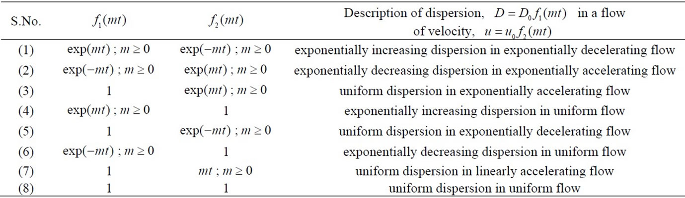
Table 1. Different combinations of temporally dependent/uniform solute dispersion and velocity of the flow.

Figure 1. Continuous curves refer to temporally increasing dispersion in decelerating flow, dashed curve refers to temporally decreasing dispersion in accelerating flow and dotted curve refers to uniform dispersion in uniform flow. Concentration values are evaluated from solution in Equation (29) for uniform input point source.

Figure 2. Continuous curves refer to uniform dispersion in accelerating flow and dashed curve refers to temporally increasing dispersion in uniform flow. Concentration values are evaluated from solution in Equation (29) for uniform input point source.

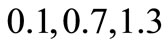
Figure 3. Continuous curves refer to uniform dispersion in decelerating flow and dashed curve refers to temporally decreasing dispersion in uniform flow. Concentration values are evaluated from solution in Equation (29) for uniform input point source.
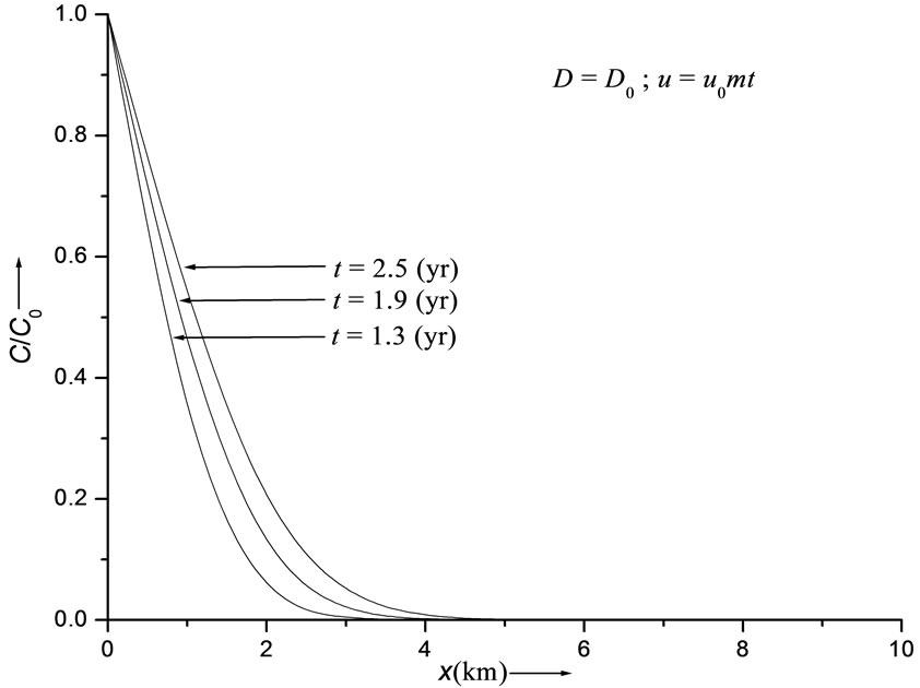
Figure 4. Concentration values evaluated from solution in Equation (29). Curves refer to uniform dispersion in linearly accelerated flow.
transport pattern for the temporally dependent dispersion problem stated by the combination (1) of table 1. The pattern is on the expected lines, i.e., in the presence of uniform point source of pollution the concentration level decreases with position at a time and increases with time at a particular position. This solution is compared with two other solutions obtained for the combinations (2) and (8), respectively at 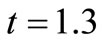 (years). Thus the concentration distribution behaviors in cases of increasing dispersion in decelerating flow; decreasing dispersion in accelerating flow; and uniform dispersion in uniform flow, are compared with each other. It may be observed that the concentration values in the combination (8) occur in between the concentration values in other two combinations, those for the combination (2) being the least. It means in case of decreasing dispersion in an accelerated flow field the concentration will reach the danger level in a region away from the source of the pollution, in the longest time. The solid curves in Figure 2 represent the solution (29) of the dispersion problem described by the combinations (3) at the three times mentioned at the outset of this section. One curve of this combination is compared with the curve drawn for the combination (4), at
  (years). It may be observed that the concentration level in case of uniform dispersion in accelerating flow domain is lower than that in case of increasing dispersion in uniform flow. Figure 3 depicts the solution (29) representing the combination (5) by the three solid curves and the combination (6) by the single dotted curve. It shows that the concentration level at a particular time
  (years) in case of uniform dispersion in a decelerating flow is higher than that in case of decreasing dispersion in an uniform flow. This trend will be same at all times but the difference between concentration values of the two combinations decreases with time more evidently in the middle region of the considered domain. Figure 4 depicts the concentration values obtained from the solution in Equation (29) for uniform dispersion along a time dependent flow domain in which velocity increases linearly defined by the combination (7). It may be noted that the expression
 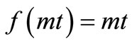 cannot be used for
 . The solute distribution pattern in this case being much slower as compared to those obtained for the other combinations considered above. As evident from Equation (15) the solution in equation (29) cannot be traced for
 ,
,  but the solutions in Equations (30-31) can be used to trace this case (the figure is not drawn). From Figures (1-3) it may be observed that at a particular position at
 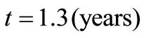 the concentration values for the combinations (1), (4), (5), (8), (3), (6), and (2) are in decreasing order.
Figure 5 depicts the concentration distribution behavior of increasing input point source described by the solution in Equation (40) for the combination (1) by the solid curves for the same input values but in a shorter
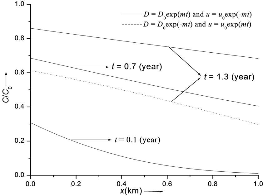
Figure 5. Continuous curves refer to temporally increasing dispersion in decelerating flow and dotted curve refers to temporally decreasing dispersion in accelerating flow. Concentration values are evaluated from solution in Equation (40) for input point source of increasing nature.
domain 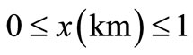 at lesser times
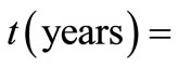
 . The solution for this input for the combination (2) is also depicted in the same figure at
  by the only dotted curve. It may be observed that concentration values for the latter combination at
  are less than those for the former combination. It may be noted that the input concentration
 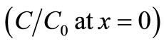 increases with time as demanded by the condition in Equation (32). The solute transport pattern is same as in case of the uniform input. The solution for the latter combination may be obtained by replacing
  by
by  in the solution in Equation (40) but in that solution the expressions for the new independent variables will be
 , and
, and .
.
4. Conclusions
There is growing concern in understanding and evaluating the pollutants solute particles transport along the medium due to diffusion and advection degrading the hydro-environment. It is important to solve advectiondiffusion equation in real cases. In that order this equation in one-dimension is solved for a general case of temporally dependent dispersion along temporally dependent flow where dispersion is not proportional to the velocity, with respect to a homogeneous first type initial condition, non-homogeneous first and third type input conditions, respectively and homogeneous flux type condition at the far end of the semi-infinite medium. The solutions for other cases of temporally dependent dispersion along uniform flow; uniform dispersion along unsteady flow and uniform dispersion along uniform flow, are obtained as particular cases. The analytical solutions in each of the four cases are compared with each other. A clear distinction between them may be observed from the figures. Two functions one exponentially increasing with time and other exponentially decreasing with time are considered for the purpose. The present study establishes that among all the possibilities considered the degradation of a water domain in slowest in case of the decreasing solute dispersion in an accelerated flow domain. It is slightly better than that in case of decreasing dispersion in uniform flow. It has also been established that the concentration attenuation in a semi-infinite medium is faster than that in a finite medium (Kumar et al., [22]). So a position farther away from the source in a semi-infinite medium is safe for longer period of time. Relying upon such studies the reason of low concentration levels may be thought of, enforcing which technologically or by other means degradation of hydro-environment may be controlled. The similar dispersion problems may be solved analytically in cases of pulse type input condition and initial spatial distribution described by Fischer et al. [23].
5. Acknowledgements
This work is part of the Post Doctoral Fellowship program of first two authors. Financial assistance provided by the funding agency to first author in the form of Dr. D. S. Khothari Post Doctoral Fellowship, University Grant Commission and second author in the form of NBHM Post Doctoral Fellowship, Department of Atomic Energy, Government of India, are gratefully acknowledged.
REFERENCES
- A. Ogata and R. B. Banks, “A Solution of the Differential Equation of Longitudinal Dispersion in Porous Media,” US Geological Survey Professional Papers, No. 34, 1961, p. 411-A.
- D. R. F. Harleman and R. R. Rumer, “Longitudinal and Lateral Dispersion in an Isotropic Porous Medium,” Journal of Fluid Mechanics, vol. 16, No. 3, 1963, pp. 385- 394. doi:10.1017/S0022112063000847
- V. Guvanasen and R. E. Volker, “Experimental Investigations of Unconfined Aquifer Pollution from Recharge Basins,” Water Resources Research, vol. 19, No. 3, 1983, pp. 707-717. doi:10.1029/WR019i003p00707
- T. J. Marshal, J. W. Holmes and C. W. Rose, “Soil Physics,” 3rd Edition, Cambridge University Press, Cambridge, 1996.
- R. B. Banks and J. Ali, “Dispersion and Adsorption in Porous Media Flow,” Journal of Hydraulic Division, vol. 90, No. 5, 1964, pp. 13-31.
- A. Ogata, “Theory of Dispersion in Granular Media,” US Geological Survey Professional Papers, No. 411-1, p. 34, 1970.
- S. H. Lai and J. J. Jurinak, “Numerical Approximation of Cation Exchange in Miscible Displacement Through Soil Columns,” Soil Science Society American Proceeding, vol. 35, No. 6, 1971, pp. 894-899. doi:10.2136/sssaj1971.03615995003500060017x
- M. A. Marino, “Distribution of Contaminants in Porous Media Flow,” Water Resources Research, vol. 10, No. 5, 1974, pp. 1013-1018. doi:10.1029/WR010i005p01013
- A. N. S. Al-Niami and K. R. Rushton, “Analysis of Flow against Dispersion in Porous Media,” Journal of Hydrology, vol. 33, No. 1-2, 1977, pp. 87-97. doi:10.1016/0022-1694(77)90100-7
- M. Th. van Genuchten and W. J. Alves, “Analytical Solutions of the One Dimensional Convective-Dispersive Solute Transport Equation,” US Department of Agriculture, Technical Bulletin, No. 1661, 1982.
- F. T. Lindstrom and L. Boersma, “Analytical Solutions for Convective Dispersive Transport in Confined Aquifers with Different Initial and Boundary Conditions,” Water Resources Research, vol. 25, No. 2, 1989, pp. 241-256. doi:10.1029/WR025i002p00241
- D. K. Jaiswal, A. Kumar, N. Kumar and R. R. Yadav, “Analytical Solutions for Temporally and Spatially DePendent Solute Dispersion of Pulse Type Input ConcenTration in One-Dimensional Semi-Infinite Media,” Journal of Hydro-Environment Research, vol. 2, 2009, pp. 254-263. doi:10.1016/j.jher.2009.01.003
- A. Kumar, D. K. Jaiswal and N. Kumar, “Analytical Solutions to One-Dimensional Advection-Diffusion Equation with Variable Coefficients in Semi-Infinite Media,” Journal of Hydrology, vol. 380, No. 3-4, 2010, pp. 330-337. doi:10.1016/j.jhydrol.2009.11.008
- S. R. Yates, “An Analytical Solution for One Dimensional Transport in Porous Media with an Experimental Dispersion Function,” Water Resources Research, vol. 28, No. 8, 1992, pp. 2149-2154. doi:10.1029/92WR01006
- J. D. Logan and V. Zlotnik, “The convection-Diffusion Equation with Periodic Boundary Conditions,” Applied Mathematics Letter, vol. 8, No. 3, 1995, pp. 55-61. doi:10.1016/0893-9659(95)00030-T
- J. D. Logan, “Solute Transport in Porous Media with Scale-Dependent Dispersion and Periodic Boundary Conditions,” Journal of Hydrology, vol. 184, No. 3, 1996, pp. 261-276. doi:10.1016/0022-1694(95)02976-1
- M. M. Aral and B. Liao, “Analytical Solutions for TwoDimensional Transport Equation with Time-Dependent Dispersion Coefficients,” Journal of Hydrologic Engineering, vol. 1, No. 1, 1996, pp. 20-32. doi:10.1061/(ASCE)1084-0699(1996)1:1(20)
- R. Haberman, “Elementary Applied Partial Differential Equations,” Prentice-Hall, Englewood Cliffs, 1987.
- G. Matheron and G. De Marsily, “Is Transport in Porous Media Always Diffusive, a Counterexample,” Water Resources Research, vol. 16, No. 5, 1980, pp. 901-917. doi:10.1029/WR016i005p00901
- G. Sposito, W. A. Jury and V. K. Gupta, “Fundamental Problems in the Stochastic Convection-Dispersion Model for Solute Transport in Aquifers and Field Soils,” Water Resources Research, vol. 22, No. 1, 1986, pp. 77-88. doi:10.1029/WR022i001p00077
- L. W. Gelhar, C. Welty and K. R. Rehfeldt, “A Critical Review of Data on Field-Scale Dispersion in Aquifers,” Water Resources Research, Vol. 28, No. 7, 1992, pp. 1955-1974. doi:10.1029/92WR00607
- A. Kumar, D. K. Jaiswal and N. Kumar, “Analytical Solutions of One-Dimensional Advection-Diffusion Equation with Variable Coefficients in a Finite Domain,” Journal of Earth System Science, vol. 118, No. 5, 2009, pp. 539-549. doi:10.1007/s12040-009-0049-y
- H. B. Fischer, E. J. List, R. C. Y. Koh, J. Imberger and N. H. Brooks, “Mixing in Inland and Coastal Waters,” Academic Press, New York, 1979.