Journal of Water Resource and Protection
Vol. 2 No. 3 (2010) , Article ID: 1497 , 8 pages DOI:10.4236/jwarp.2010.23029
Measuring Salinity within Shallow Piezometers: Comparison of Two Field Methods
I.G.R.G, University of Bologna, Via San Alberto, Ravenna, Italy
E-mail: balugani.enrico@libero.it, m.antonellini@unibo.it
Received December 21, 2009; revised January 14, 2010; accepted January 26, 2010
Keywords: Coastal Aquifer, Salt-Water Intrusion, Piezometers, Monitoring
ABSTRACT
The objective of this study is to understand the validity of salinity vertical profiles collected from shallow piezometers that are not previously flushed. This study shows that salinity data collected from boreholes are only an average value along the entire screened section of the piezometer. In order to collect data that is representative for the salinity of the adjacent aquifer, a new monitoring strategy has been developed. This strategy includes measurement of the salinity at the top of the watertable in an auger hole which is a shallow boreholes made with an handheld drill. This should be combined with measurements in piezometers that are first flushed to take out stagnant water. From the piezometers on can measure the average salinity of the screened part and the salinity at the bottom of the aquifer. By using this monitoring strategy it is also possible to define where the piezometers screens are located if this is not known beforehand.
1. Introduction
1.1. Overview
A large part of the world population lives along the coasts exerting a strong pressure on freshwater resources [1]. Overexploitation of coastal groundwater often results in subsidence and saltwater intrusion. The area considered in this study is part of the Po Plain coast, particularly affected by salt-water intrusion problems, because of the low topography with respect to sea level and the anthropogenic pressure connected to tourism, agriculture, and the gas industry [2]. Italy is one of the countries most affected by saltwater intrusion, due to the relatively high population density (196,6 inhabitants/km2) and the length of its coastline (more than 8000 km). To the best of our knowledge, a standard monitoring methodology and protocols to characterize this phenomenon has not yet been developed, so that approaches in different areas of the world may be quite different according to local knowledge of the saltwater intrusion problem. There are different approaches to study saltwater intrusion in coastal aquifers, for example geophysical methods [3], borehole investigations, and numerical models [4]. Borehole data are widely used in these kinds of studies, especially for calibrating numerical models, but in recent years the validity of data collected directly from wells and piezometers is under discussion [5–9]. Characterizing piezometric heads and salinity within a large coastal phreatic aquifer is a complex endeavour. The point water head measured in a salty aquifer needs to be corrected and transformed to equivalent freshwater head or environmental head [10] in order to have a correct representation of the hydraulic gradients. As pointed out by the numerical experiments described in [9], the salinity measured in a borehole or a piezometer, that happens to be in the mixing zone of a coastal aquifer, may not be representative for the fluids within the porous medium. In long-screened boreholes, preferential flow within the borehole (Figure 1), driven by gradients in concentration, results in biased data for groundwater samples or measurements collected from the well-water profile [9]. These data have poor relationships with the effective environmental concentrations of chemicals [6]. Flow in the borehole (Figure 1) does not only affect the chemical concentrations in the well, but also affects the near-borehole aquifer acting as a preferred flow channel for solutes [11–13]. Shallow conventional wells and piezometers are, especially, prone to this problem [14]. The reliability of data collected from boreholes is strongly connected to the length of the screened section; the longer the screen the greater the bias [14]. From Britt's experiments [8] it is clear that the assumption of
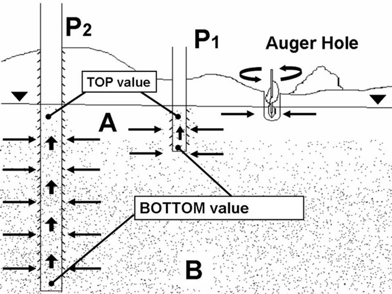
Figure 1. Hypothesis on salt distribution inside and near the piezometer, based on Britt (2005) and Elci et al. (2001). P1 = type 1 piezometer; P2 = type 2 piezometer; A = fresh water; B = salt water; points represent salt, arrows represent the directions of salt movement.
linear flow in a piezometer under normal conditions is questionable.
1.2. Objective of the Study
This paper presents field measurements of watertable elevation and salinity made with two different methods in shallow wells within a coastal phreatic aquifer. Our study site, the San Vitale pine forest, is strongly affected by saltwater intrusion [2,15], and the monitoring system in place since the last fifteen years consists of more than 20 conventional piezometers 6,4 cm in diameter, with a screen along their whole length (Figure 1); the monitoring system used so far (method A) is based on salinity measurements from conventional shallow piezometers without flushing the stagnant water. A four year long collection of monthly data already exists for this area (starting from 2004). Given the importance of past data in the study of the evolution of saltwater intrusion along the coast, we decided to find a way to test their validity in view of their integration with measurements from current and future surveys. The specific objectives of this study were to understand how the borehole-flow related bias affects salinity measurements collected during sampling in a piezometer network within a phreatic aquifer, what exactly the data represent, infer the validity of the data collected during the past years and to develop an appropriate method of sampling. This has been done by means of field experiments on the existing piezometers, by comparison with previously collected data (method A - CTD probe and no flushing), and by drilling auger holes to the top of the watertable combined with salinity measurements in flushed piezometer (method B). Another objective of the study was to assess the position of the screens along existing boreholes in the phreatic aquifer that for some piezometers was not reported before.
1.3. Setting
Our study area is located in the San Vitale pine forest, north of Ravenna, on the north Adriatic coast of Italy. The area borders on the south with the city of Ravenna, on the north with the Destra Reno canal (not shown), on the west with two freshwater wetlands (Boundary Water Bodies, in Figure 2), on the south with the Romea highway (S.S. 309), and on the east with farmland and the Piallassa Baiona lagoon (B.W.B. on the right in Figure 2). This latter lagoon is divided by dikes in several water bodies and is partly connected to the sea: the westernmost water bodies have been closed and remain filled with freshwater, whereas those in the east have salinity similar to that of the sea and experience tide-induced water level fluctuations. The area is covered by a pine forest planted by the Romans on paleodunes with belts that run in a north–south direction. The surface hydrographic system consists of east-west oriented river and channels, open surface water bodies, and drainage ditches with pumping machines that discharge water towards the sea. The area is undergoing subsidence due to natural and anthropogenic causes; the subsidence has dropped most of the forest below mean sea level [15,16]. Soils are mostly sandy and their specific characteristics depend on morphology and watertable depth. The area stratigraphy is consists of multiple series of transgressive-regressive deposits [17–20]. These sediments forming the aquifers are composed of clay layers
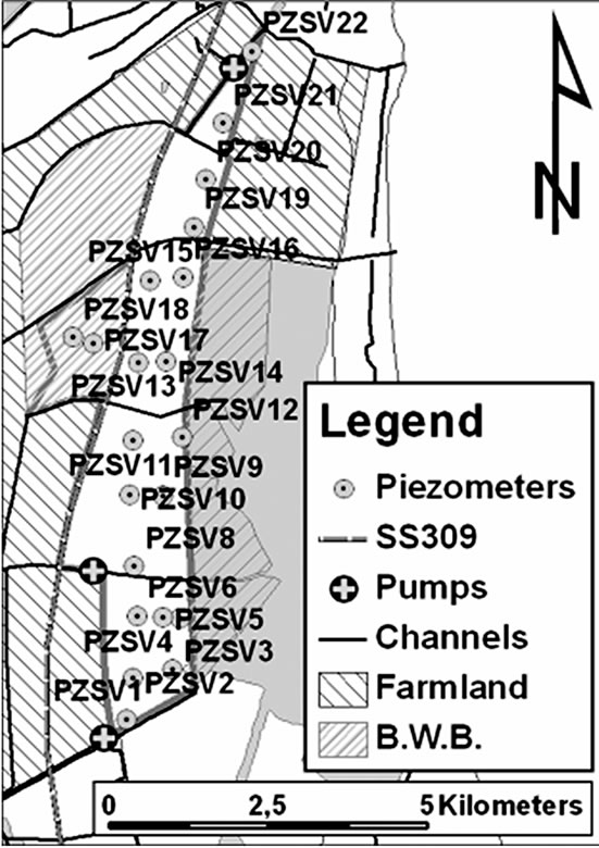
Figure 2. Detail of the study area with boundaries and piezometers location (called PZ), rivers and canals, water bodies and wetlands in proximity to the San Vitale pine forest. B.W.B. stands for Boundary Surface Water Bodies.
(aquiclude) stratified with sand layers (Figure 3). The phreatic aquifer corresponds to the upper sand layer; it is confined at the bottom by a clay-silt and sand-silt unit that acts as aquiclude (from -10 m to -21 m) [21]. The aquifer hydraulic conductivity (K) is known by slug tests [2,22], the range in K vary between 14 and 30 m/day [22]. Depth of watertable from the surface ranges from 0 to -4 m. The piezometer network covers the whole pine forest area with an irregular grid: the maximum distance between two piezometers is 1 km, and the minimum is 200 m. All piezometers are in the forested area except PZ17 and PZ18, that are located in the Punte Alberete wetland (Figure 2).There are two types of piezometers (Figure 1): the first one consists of short piezometers (type 1; PZ4, 5 and 6) that are 3 m long and have 3,8 inch diameter whereas the second one (type 2) consists of piezometers that are 6 m long and have a 6,4 inches diameter. The total length of the screen in these piezometers is unknown. The common procedure in the area was to screen the last meter of the short piezometers (type 1) and to screen completely the long piezometers (type 2).
2. Methods
Until now, the monitoring procedure (method A) used in our study area consisted of watertable head, electric conductivity, and temperature measurements directly in the piezometers by means of a CTD probe (AQUATroll®200) that records a profile of these parameters in each piezometer. The piezometers were not flushed by pumping before the measurements were made. Electrical conductivity data are then converted into salinity values using the equations by Lewis & Perkins [23]. Watertable level data were measured with a standard water-level meter (resolution: 1 cm). The new method (method B) uses a different approach; in order to reduce the bias due to stagnant water above the screens, we decided to flush away from the piezometer a water quantity equivalent to 3 wet borehole volumes [24] and to measure the electric conductivity and temperature at the top and bottom of the piezometer. Pumping has been conducted from the top of the watertable (see Figure 1) at an approximate rate of 4 liters per minute.
In this way, we collected two different types of information:
1) from the difference between top and bottom salinity (see Figure 1) we infer the length of the screened section 2) from the electrical conductivity data recorded post-flushing we obtain a more representative average salinity value for the part of the aquifer in contact with the bottom of the piezometer.
A large difference between top salinity before and after flushing occurs in piezometers that are screened only in the last bottom meter because stagnant water is removed and replaced with ground water coming from the screened section.
However, a small difference occurs in piezometers that are fully screened, because there is less stagnant water.
After this, we compared the salinity measured within the borehole with that in the adjacent aquifer. The salinity at the top of the watertable was obtained by digging a shallow auger hole (5 cm deeper than the watertable, just to submerge the probe; Figure 1) near the piezometer (distance between 5 to 20 m) to reach the watertable top and take measurements of electric conductivity and temperature.
The experiment has been conducted in three days distributed within two weeks from 6 to 15 august 2008 without any rainfall event. The water extracted was red to brown colored (iron oxides in the water from the steel casing) at the beginning of the pumping, and then turned clear once the stagnant water was flushed away.
In order to better evaluate the results of the experiment, the problem has been simplified by dividing the area into subareas bordered by natural hydrologic boundaries, such as rivers or canals.
3. Result and Discussion
The results of our monitoring campaign show that the watertable levels are below or equal to the mean sea level in the whole area (Table 1). Groundwater levels are close to 0 m msl in the southeastern part of the aquifer and in its northwestern part. The regions where the interpolated water table is close to 0 m msl correspond to the boundaries of surface water bodies. The lowest watertable level is -2,22 m msl and it has been observed in the northern part of the forest at piezometer SVPZ21. The highest watertable level is 0.02 m and it has been observed in the central part of the forest at PZSV17.
The measurements done in piezometers 1, 4, 5, 6, 8, 10, 11, 13, 18, 20, 22. before flushing show a salinity at the top of the watertable below 1,5 g/l which is the limit salinity for fresh water; [25] The salinity measured at the bottom of the piezometers before flushing ranges from 6 to 27 g/l in the southern area (piezometers from
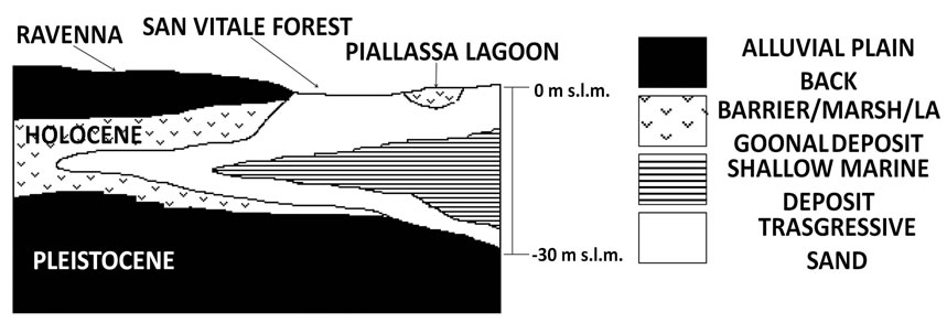
Figure 3. Schematic stratigraphic reconstruction of the coastal aquifer below the study area (modified after Amorosi et al., 1999 and Marchesini et al., 2000).
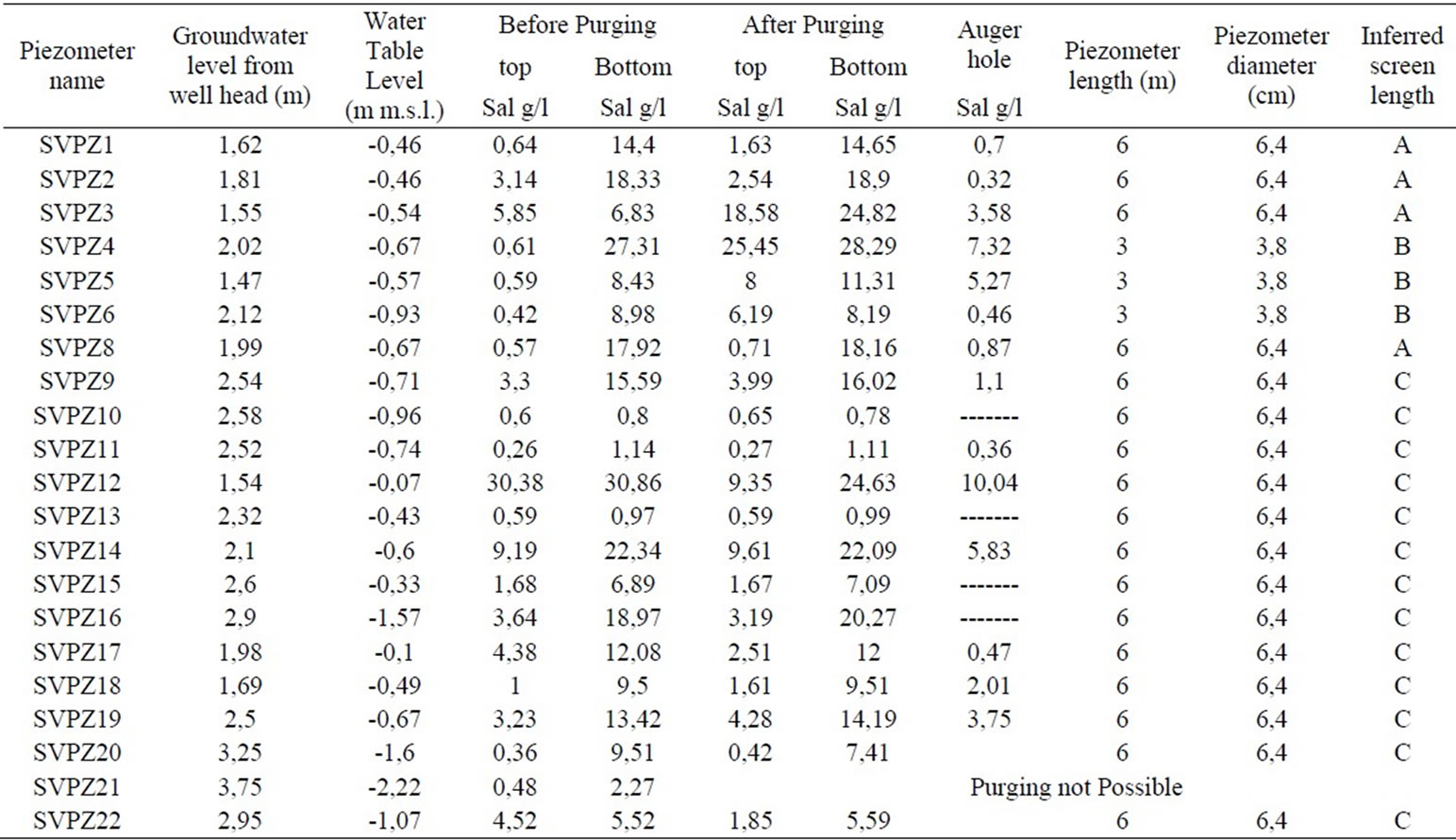
Table 1. Salinity and groundwater level data measured in piezometers before and post-flushing the stagnant water during this study.
1 to 6), from 2 to 13 g/l in the northern area (piezometers from 19 to 22), and is rather variable in the central area (salinity values range from 0.8 to 31 g/l). After flushing away the stagnant water, the salinity values at the top of the watertable in the piezometers remain below 1,5 g/l in boreholes 8, 10, 11, 13, 20. The salinity measured at the bottom of the piezometers post-flushing the stagnant water, ranges from 8 to 28 g/l in the southern area, from 5 to 14 g/l in the northern area, it is about 10 g/l in Punte Alberete, and it varies between 0,8 to 25 g/l in the central area.
The salinity measured in the Auger holes is below 1,5 g/l next to piezometers 1, 2, 6, 8, 9, 11, 13, 17 and it is above 5 g/l next to piezometers 4, 5, 12, 14 (again, Table 1).
3.1. Data Analysis
The watertable levels have not changed after pumping for flushing the stagnant water. This is due to the high hydraulic conductivity of the aquifer (K = 14 - 30 m/d, [2]). The highest watertable levels (0.02 m in PZSV17) have always been observed in proximity to open surface water bodies, such as the Piallassa lagoon in the south (Figure 3). The different gradients cause two main groundwater fluxes: one from west to east in the northern part of the study area, and one from west and south to the northwest in the southern part.
3.1.1. Measurements at Top of the Watertable
We compared the salinity at the top of the watertable measured in the piezometers with that measured in the auger holes. The salinity measurements at the top of the watertable within the piezometers, collected during our study campaign before flushing the stagnant water (Table 1), are similar to the previous measurements collected in the same season during 2007 (Table 2). It appears that the salinity remained more or less the same in the central and northern parts, with the exception of piezometer 12 where the salinity is higher than it was before (16,39 g/l during 2007, 30,38 g/l during 2008, see Tables 1 and 2) and decreased (from 22 g/l to 0.5 g/l in PZSV4) in the southern part of the forest. Post-flushing (Figure 4), the situation changes. The largest variations with respect to pre-flushing salinity occur in piezometer 12 (decrease in salinity of 21,03 g/l) and in the southern part of the area where the salinity decreases (for all piezometers, differences in salinity are more than 100 %, see Table 1). In some cases the saltwater-freshwater interface is apparently so close to the bottom of the piezometer that flushing the stagnant water causes up-coning of seawater. This is shown in piezometer 4, where before pumping there was a fresh-water lens (salinity 0.61 g/l), and after pumping the salinity increased to 35 g/l. The observed variation in salinity values induced by pumping are related to two different factors: the first one is the different response of wells to pumping due to differences
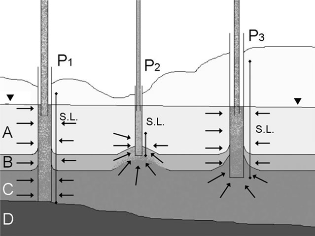
Figure 4. Different borehole behaviour in response to pumping. In a fully penetrating borehole the laminar flux from the aquifer remains mainly horizontal, whereas in incomplete penetrating well a vertical flow component is present. P1 = type 1 piezometer; P2 = type 2 piezometer, fully penetrating; P3 = type 2 piezometer, partially penetrating; D = aquifer bottom; S.L. = screen length. Arrows represent water flow directions.
in length of the piezometers and position of the screens, on which depends the amount of stagnant water before pumping and the level from which groundwater flows into the piezometer during pumping, the second one is natural mixing with saltwater due to up-coning where the freshwater-saltwater interface is in close proximity to the bottom of the piezometer. The salinity measured in the auger holes (or auger drills, Figure 1) is generally lower than that measured in the piezometers (mean difference is 1,58 g/l). The salinity measurements made in the auger holes remain high near the Piallassa lagoon, but they are 10 or more g/l lower than what was measured in the piezometers (Table 1).
3.1.2 Measurements at bottom of piezometers
The salinity measurements at the bottom of the piezometers (6 m c.a.), that we made in this study before flushing the stagnant water, fit well to the data collected in previous years [22] and the local public records (Table 2); the only relevant variation from previous years is in the southern part, between the two pumps shown in Figure 2. In this latter area, the salinity in piezometers PZSV3, PZSV4 and PZSV8 is less than what was measured previously (5 % of mean difference – see Tables 1 and 2). After pumping, the salinity varies with respect to the pre-pumping data; in the northern and central part of the forest the differences are minimal, in the northeastern part (piezometers 16, 19, 20), the salinity decreases after pumping.
3.2. Interpretation of Salinity Changes
The salinity measured after pumping was interpreted using the work described in [24] on wellbore responses to pump-induced flow and mixing in controlled laboratory conditions. Our idea was to interpret field salinity profile variations in wells due to pumping in controlled conditions for different well screen lengths in a way to relate these variations to different well geometries. Differences between the situation before and after pumping vary widely from piezometer to piezometer. Bottom salinity measured after pumping is always higher than bottom salinity measured before pumping, whereas the top watertable salinity measurements are sometimes higher and sometimes lower with respect to pre-pumping value. The distribution in variations among salinity measurements preand after pumping show that the San Vitale pine forest can be divided into two areas: the northcentral one and the southern one (Figure 3). In the southern area piezometers of type 1 (3 piezometers) and 2 (4 piezometers) are present and the cause of the differences in salinity is likely the different lengths of the screens in the two types of piezometers. In the northern area, the salinity at both top and bottom is the same regardless of the monitoring method, therefore also previous measurements made without flushing could be considered to be representative for the aquifer. In the central-northern area, all piezometers have the same geometry; differences between top-piezometer and auger hole salinity data increase slowly at increasing salt concentration (Difference for PZSV14 was 36 %; for PZSV22 was 10,6 %). There are also small differences (mean 1 g/l) in salinity measured in piezometers from the northern area before and after-flushing and in auger holes (Table 1). This suggests that the screen length coincides with the total length of the piezometer .The salinity data measured in the piezometers at the top of the watertable in the northern area are similar to those measured in the auger-holes, because the aquifer is in connection with the screened profile. The mean difference between the salinity measurements collected at the top of the watertable post-flushing and in auger holes for the southern area is over 1000 % (7,46 g/l) for the type 1 piezometers. Differences between the salinity at the top of the piezometers before and postflushing for piezometers 12 and 22 are difficult to understand: a possible explanation for piezometer 12 could be the relatively high watertable (1,54 m from well head, whereas all others have a watertable deeper than 2 meters from the well head) and proximity to water body that is influenced bu the tides, resulting in strong well mixing caused by water level fluctuations in the piezometer [9]. Differences between auger holes measurements and piezometers measurements show no apparent relationships with other variables such as borehole geometry, morphology, vegetation, proximity to water bodies, and lithology. We conclude that type 2 piezometers are screened from 2 to 6 meters from the borehole head, so that they can be interpreted to be fully penetrating (P2 in Figure 4) the phreatic aquifer in the northern area of the pine forest where the depth of the bottom acquiclude is at a depth between -6 and -7 m [2].
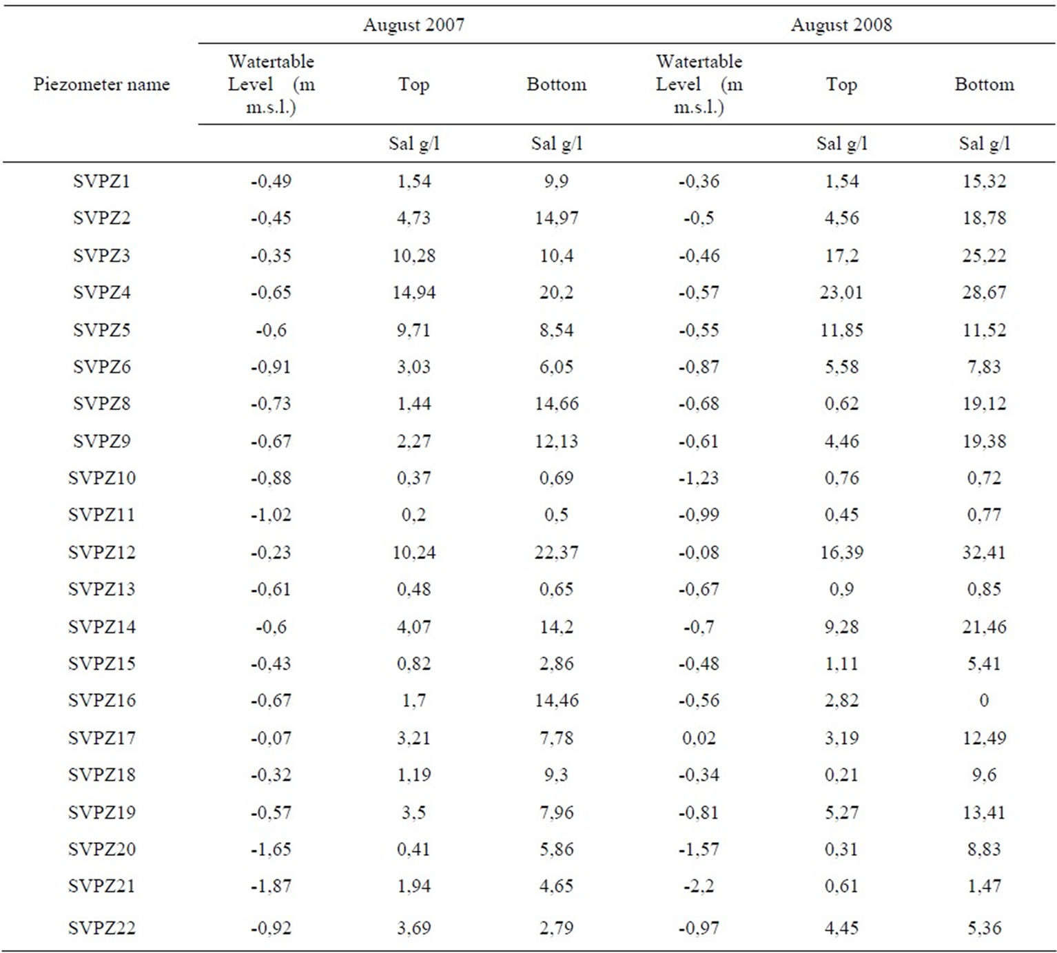
Table 2. Salinity and watertable level measurements in piezometers for the months of August 2007 and 2008.
In the southern area, differences between bottom salinity data before and after pumping show a dual behaviour (Table 1): salinity measurements in piezometers 1, 2 and 6 remain unchanged, whereas in the other piezometers they change significantly (mean difference of 100 % salinity for PZSV3, 4 and 5, respectively). This suggests that the differences are not related to borehole geometry. In the southern area, the electric conductivity profiles made before pumping, suggest that the driving factor controlling bottom salinity data variations should be proximity to the saltwater of the Piallassa lagoon (Figure 2): the borehole bottom remains just above a sharp interface between freshwater and saltwater and during pumping, saltwater up-coning takes place causing strong mixing in the piezometer (Figure 4). The differences in top watertable salinity measured before and after pumping have a similar pattern to the bottom salinity differences previously described: piezometers 1 and 2 show small differences (0,98 and 0,6 g/l, respectively) whereas, for the other piezometers in the southern area, top salinity values change considerably (7 % for PZSV3, 4, 5 and 6, respectively). This shows that borehole screen length is different in the two types of piezometers belonging to the two network sets. The type 1 piezometer is screened only in the last meter: this explain both similarity between bottom salinity values before and after pumping and the marked difference between top salinity values before and after pumping.
Few of the salinity values at the top of the piezometers measured after pumping are close to those measured in the auger holes (Table 1): this shows that effective groundwater density stratification is lost in boreholes, because of internal fluxes and mixing.
The large difference in salinity (see Tables 1 and 2) between the two measurement methods (A and B) in both northern and southern areas could be the depth of the clay aquiclude. In the northern and central area the piezometers are almost completely penetrating, because the depth of the aquiclude and the length of the piezometer coincide (6 m). In the southern area, however, the clay layer at the bottom of the aquifer is at a depth that is twice the piezometer’s length (13 m). For this reason, at the bottom of the piezometer, fluxes occur in both an horizontal and vertical direction and there is vertical seepage of saltwater into the piezometer (Figure 4 [26]).
3.3. Determination of the Position and Length of the Screen
A study of the piezometers/well response to pumping, like the one we performed in this study, could be used to determine the position and length of the screens if such position and length are not known. This requires also knowledge of the aquifer’s thickness in order to avoid the use of partially penetrating piezometers. If the groundwater at the top of the aquifer is sampled using the auger holes method, and a salinity profile is measured along the piezometers before and after pumping, the comparison between the field data and the numerical models for different screen/length configurations [13] allows to infer the position and length of the screened section (our results have been confirmed by using a straddle-packer multilevel system on the same piezometers).
This study shows that the use of partially penetrating piezometers should be avoided in monitoring acquifer salinization. Auger holes, on the contrary, seem a reliable way to obtain representative data about the salinity at the top of the groundwater. Fully penetrating and screened piezometers could be used to obtain the average water salinity data through the whole aquifer column after proper flushing of the stagnant water. More representative values for groundwater salinity at different depths could only be obtained by using cluster piezometers or multilevel samplers.
4. Conclusions
The salinity measurement method used in this study has certain advantages in characterizing the salinity at the top of the watertable and it has allowed us to critically evaluate salinity values measured before in previous studies that did not include flushing the wells.
If the piezometer is not fully penetrating, measurement obtained is an average comprehensive of deeper parts of the aquifer. Surface groundwater salinity obtained by auger holes measurements is considerably lower than what expected from the piezometers data.
Our study has shown that it is important, in the design of networks to monitor salinity, that piezometers are fully penetrating and screened through the aquifer of interest.
We have also developed a methodology to indirectly assess the length and position of the screened section of the piezometers for which no record is available. With this method it is, therefore, possible to obtain information about the screened section of old piezometers already present in an area and use them in a hydrogeology study.
5. Acknowledgment
We thank the Municipality of Ravenna and a strategic funding project of the University of Bologna for financial support. We thank also V. Marconi for the field help and the inspired suggestions. The revision of P. Mollema helped to improve this manuscript.
REFERENCES
- T. Beatley, D. J. Brower, and A. K. Schwab, “An introduction to coastal zone management,” Published by Island Press, 2002.
- M. Antonellini, P. Mollema, B. Giambastiani, K. Bishop, L. Caruso, A. Minchio, L. Pellegrini, M. Sabia, E. Ulazzi, and G. Gabbianelli, “Salt water intrusion in the coastal aquifer of the southern Po Plain, Italy,” Hydrogeology Journal, Vol. 16, No. 8, December 2008.
- S. S. A. Nassir, M. H. Loke, C. Y. Lee, M. N. M. Nawawi, “Salt-water intrusion mapping by geoelectrical maging surveys,” Geophysical Prospecting, Vol. 48, pp. 647–661, 2000.
- O. E. GHP, “Salt water intrusion in a three-dimensional groundwater system in the Netherlands: a numerical study,” Transp Porous Media, Vol. 43, No. 1, pp. 137– 158, 2001.
- R. M. Powell and R. W. Puls, “Passive sampling of groundwater monitoring wells without purging: Multilevel well chemistry and tracer disappearance,” Journal of Contaminant Hydrology, Vol. 12, No. 1–2, pp. 57–77, 1993.
- P. E. Church and G. E. Granato, “Bias in groundwater data caused by well-bore flow in long-screen wells,” Ground Water, Vol. 34, No. 2, pp. 262–273, 1996.
- J. M. Martin-Hayden and G. A. Robbins, “Plume distortion and apparent attenuation due to concentration averaging in monitoring wells,” Ground Water, Vol. 35, No. 2, pp. 339–346, 1997.
- L. S. Britt, “Testing the in-well horizontal laminar flow assumption with a sand-tank well model,” Ground Water Monitoring & Remediation, Vol. 25, No. 3, pp. 73–81, 2005.
- E. Shalev, A. Lazar, S. Wollman, S. Kington, Y. Yechieli, and H. Gvirtzman, “Biased monitoring of fresh water-salt water mixing zone in coastal aquifers, Ground Water, Vol. 47, No. 1, pp. 49–56, 2009.
- C. W. Fetter, Applied Hydrogeology, 4th ed., Upper Saddle River, Prentice-Hall, New Jersey, 2001.
- T. E. Reilly and D. R. LeBlanc, “Experimental evaluation of factors affecting temporal variability of water samples obtained from long-screened wells,” Ground Water, Vol. 36, No. 4, pp. 566–576, 1998.
- J. M. Martin-Hayden, “Sample concentration response to laminar wellbore flow: Implication to groundwater data variability,” Ground Water, Vol. 38, No. 1, pp. 12–19. 2000.
- A. Elci, F. J. Molz III, and W. R. Waldrop, “Implication of observed and simulated ambient flow in monitoring wells,” Ground Water, Vol. 39, No. 6, pp. 853–862, 2001.
- S. R. Hutchins and S. D. Acree, “Ground water sampling bias observed in shallow, convenional wells,” Ground Water Monitoring and Remediation, Vol. 20, No. 1, pp. 86–93, 2000.
- B. M. S. Giambastiani, M. Antonellini, G. H. P. Oude Essink, R. J. Stuurman, “Saltwater intrusion in he unconfined coastal aquifer of Ravenna (Italy): A numerical model,” Journal of Hydrology, Vol. 340, pp. 91–104, 2007.
- P. Teatini, M. Ferronato, G. Gambolati, and M. Gonella, “Groundwater pumping and land subsidence in the Emilia-Romagna coastland, Italy: Modeling the past occurrence and the future trend,” Water Resources Research, Vol. 42, 2006.
- M. Bondesan, G. Calderoni, and R. Dal Cin, “Il litorale delle province di Ferrara e di Ravenna (alto Adriatico), evoluzione morfologica e distribuzione dei sedimenti,” Boll Soc Geol, pp. 247–287, 1978.
- A. Amorosi, M. L. Colalongo, G. Pasini, D. Preti, “Sedimentary response to Late Quaternary sea-level changes in the Romagna coastal plain (Northern Italy),” Sedimentology, Vol. 46, pp. 99–121. 1999.
- M. Bondesan, V. Favero, and M. J. Viñals, “New evidence on the evolution of the Po delta coastal plain during the Holocene,” Quaternary International, Vol. 29/30, pp. 105–110, 1995.
- L. Marchesini, A. Amorosi, U. Cibin, A. Zuffa, E. Spadafora, and D. Preti, “Sand composition and sedimentary evolution of a late quaternary depositional sequence, Northwestern Adriatic Coast, Italy,” Journal of Sedimentary Research, Vol. 70, No. 4, pp. 829–838, 2000.
- A. Veggiani, “Le ultime vicende geologiche del Ravennate,” In: Influenza di insediamenti industriali sul circostante ambiente naturale, Studio sulla pineta di S. Vitale di Ravenna. Ed. Compositori, Bologna, pp. 48–58, 1974.
- B. M. S. Giambastiani, “Evoluzione idrologica ed idrogeologica della pineta di San Vitale (Ravenna),” Ph.D. Thesis, Bologna University, 2007.
- UNESCO, “Algorithms for computation of fundamental properties of seawater. Unesco technical papers in marine science 44,” Unesco/SCOR/ICES/IAPSO Joint Panel on Oceanographic Tables and Standards and SCOR Working Group 51, 1983.
- J. M. Martin-Hayden, “Controlled laboratory investigations of wellbore concentration response to pumping,” Ground Water, Vol. 38, No. 1, pp. 121–128, 2000.
- P. E. Wendell, “Introduction to environmental engineering and science,” Prentice Hall, 3rd ed. ISBN, No. 0–13–148193–2, 2007.
- M. S. Hantush, “Hydraulics of wells,” in Advances in Hydroscience,” Vol. 1, Ed.: V. T. Chow, Academic Press, New York, pp. 281–432, 1964.
NOTES
Identify applicable sponsor/s here. (sponsors).