Journal of Biomedical Science and Engineering
Vol.6 No.1(2013), Article ID:27447,11 pages DOI:10.4236/jbise.2013.61009
Heart valve closure timing intervals in response to left ventricular blood pressure
![]()
1Department of Biomedical Engineering, Dalian University of Technology, Dalian, China
2Department of Information and Communication Engineering, Yeungnam University, Seoul, South Korea
Email: tanghong@dlut.edu.cn
Received 13 November 2012; revised 19 December 2012; accepted 29 December 2012
Keywords: Cardiopulmonary Modeling; Systemic Hemodynamic; Pulmonary Hemodynamic; Timing of Heart Valve Closure; Heart Sounds
ABSTRACT
This article investigates the relationships between heart valve closure timing intervals and left ventricular systolic blood pressure (LVSBP). For this investigation, the cardiopulmonary system is modeled as an analog circuit, including heart chambers, the distal and proximal aorta, distal and proximal systemic arteries/veins, systemic capillaries, the vena cava, the distal and proximal pulmonary artery, distal and proximal pulmonary arteries/veins, pulmonary capillaries and physiological control of heart rate and cardiac contractibility. In this model, the ventricles, atria and arteries were modeled as advanced pressure-volume relationships. A vagal-sympathetic mechanism was adopted to simulate transient systemic and pulmonary blood pressure. Four intervals, i.e., the timing interval between mitral and aortic valve closure (TIMA), the timing interval between aortic and mitral valve closure (TIAM), the timing interval between aortic and pulmonary valve closure (TIAP) and the timing interval between mitral and tricuspid valve closure (TIMT), are further defined in a heart cycle to illustrate their relationships to LVSBP. Simulations showed that the TIMA, TIAM and TIAP have strong negative correlations with LVSBP; meanwhile, the TIMT has a slightly negative relationship with LVSBP. To further validate the relationships, 6 healthy male subjects were experimentally evaluated. The intervals were extracted from non-invasively sampled heart sound signals taken from the surface of the thorax. The experiments showed relationships consistent with those obtained by simulations. These relationships may have potential applications for noninvasively accessing LVSBP in real-time with a high time resolution of one heartbeat.
1. INTRODUCTION
Left ventricular systolic blood pressure (LVSBP) is an important hemodynamic indicator of heart function. Developing a non-invasive method of accessing LVSBP is of interest to the medical community. However, the left ventricle is concealed in the thorax. Direct measurement by a catheter inserted to the left ventricle is commonly used for a final diagnosis. A non-invasive measurement is more widely accepted in regular medical checkups. LVSBP is often approximated by the aortic pressures measured in the left upper arm using a stethoscope and a sphygmomanometer. This approximation is inexpensive and easy to perform, but it is not a real-time measurement; it may take half a minute for one measurement. Additionally, it is uncomfortable. A non-invasive, comfortable, accurate and high time resolution LVSBP measuring method is desirable. To achieve this, the authors start from the hemodynamics of the systemic and pulmonary circulation. It is known that heart valve closure results from dynamic events associated with the interactions between the valves and differential pressures on each side [1]. The systolic contraction of the left and right ventricles triggers the closures of the mitral and tricuspid valves; meanwhile, the extension triggers the closures of the aortic and pulmonary valves. Intuitively, it may be assumed that the hemodynamics of the heart chambers and arteries must vary as the contractibility of the ventricle varies. The heart valve closures may thus be delayed or shifted to an earlier time. Previous studies have tested this assumption. For example, several systolic time intervals (STIs, i.e., the total electromechanical systole, left ventricular ejection time, and pre-ejection period) have been commonly used to illustrate their relationships with left ventricular function [2,3]. STIs may respond sensitively to exercise and pharmaceutical agents. A previous study [3] revealed that STI bears a strong negative correlation with aortic systolic pressure. To access the timing of heart valve closure, acoustic vibrations received on the chest wall, known as heart sounds S1 and S2, have been commonly used in previous works as time markers [2-5]. The time-frequency features of heart sounds have been further suggested to indicate systemic and pulmonary pressure [6-9]. However, the genesis and quantitative responses of the timing of heart valve closure to hemodynamics are still unclear. The aim of this article was to investigate the relationship between LVSBP and heart valve closure timing via simulations and experiments.
This paper is organized as follows. Section 2 presents a modified cardiopulmonary model consisting of heart chambers, simplified arteries, simplified veins and a physiological mechanism to control heart rate and heart contractibility during dynamic exercise. Section 3 shows the simulation results. The experiments that were conducted are shown in Section 4 to validate the relationships. Sections 5 and 6 present the discussion and conclusions.
2. A CARDIOPULMONARY MODEL APPLIED TO ANALYZE THE TIMINGS OF HEART VALVE CLOSURE
2.1. Cardiopulmonary Model
A modified model of the cardiopulmonary system was proposed in this paper and used as a platform to study the relationship between LVSBP and heart valve closure timing differences. The model was based on previous works from the last few decades [10-12]. The nonlinear pressure-volume (P-V) mathematical description of the heart ventricular ejection function can be simple and straightforward within a physiological framework. The nonlinear model of any part of an artery or vein generally consists of three elements: resistance, modeled by a resistor; compliance, modeled by a capacitor; and inertia, modeled by an inductor. The circulatory system is thus converted to an analog circuit, as shown in Figure 1. The values of the resistors, capacitors, and inductors are given in Appendix A. The heart cycle period is determined physiologically by the vagal-sympathetic mechanism. With the support of this cardiopulmonary platform, heart valve closure timing can be defined by the differential blood pressure (BP) across the valves.
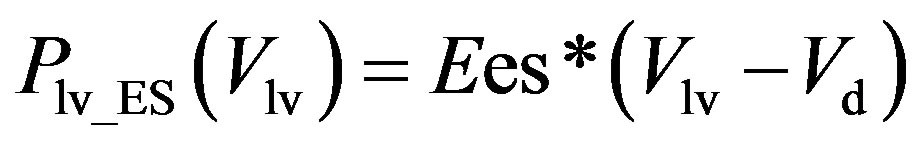
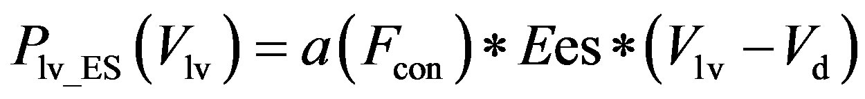
1) Ventricular model The ventricular model is based on the work of Chung et al. [13], wherein the left and right ventricles are modeled as a time-varying elastic function. The elastic function consists of three curves, i.e., the end-systolic pressure-volume relationship (ESPVR), the end-diastolic P-V relationship (EDPVR), and a time-varying activation function ev(t). For example, the blood pressure in the left ventricle, Plv, with respect to volume Vlv and time t, is given as
 (1)
(1)
 , (2a)
 , (2b)
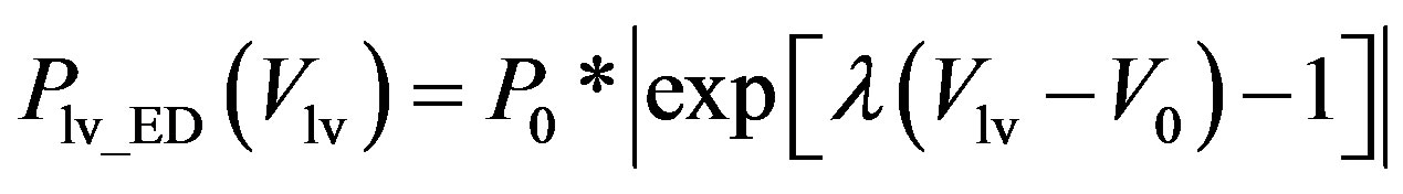
where Plv_ES(Vlv) denotes the ESPVR and Plv_ED(Vlv) denotes the EDPVR. Vd is the constant volume intercept. Ees is the end-systolic elastance. V0 is the volume inter-
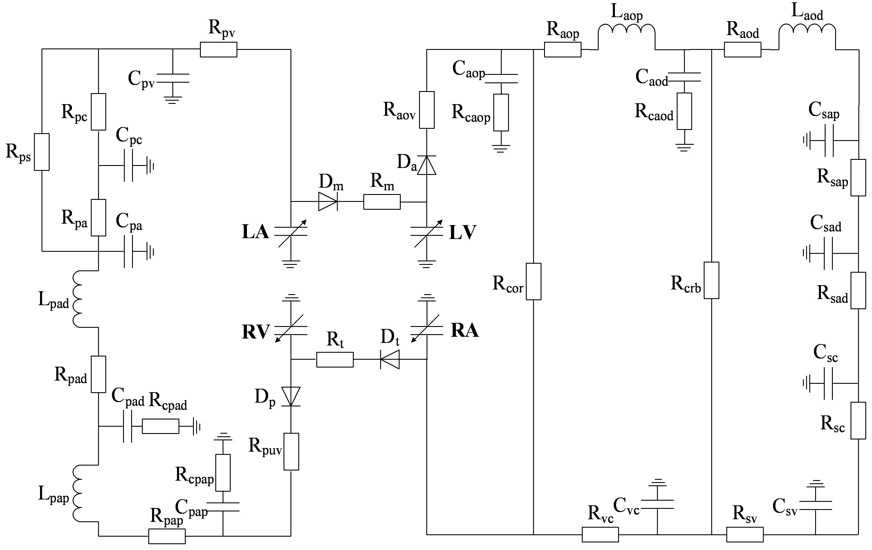
Figure 1. An analog circuit modeling the cardiopulmonary system. P: pressures; R: resistances; C: compliances; L: inertances. (Full names for the abbreviations used in subscripts can be found in Tables A1, A2 and A3).
cept for end diastole. P0 is the pressure intercept. λ is an empirical constant quantifying the P-V relationship. ev(t) is the activation function consisting of 4 Gaussian curves,
 . (3)
. (3)
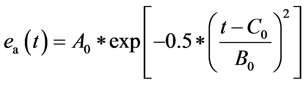
2) Atrium model The left atrium and right atrium are modeled following the same principles as those used to model the ventricles. ea(t) is the activation function consisting of one Gaussian curve,
 . (4)
. (4)
The parameters for both ventricle and atrium are given in Tables 1 and 2.
We can derive blood pressure Plv(Vlv, t), Prv(Vrv, t), Pla(Vla, t) and Pra(Vra, t) for the left ventricle, right ventricle, left atrium and right atrium, respectively, following Eqs.1 to 3. These equations have different coefficients, as illustrated in Tables 1 and 2. The parameters for Ci of the activation function used in this paper were modified according to Braunwald’s research [14]. The left ventricle contraction onset was earlier than that of the right ventricle by 13 ms; meanwhile, the right atrium contraction onset was earlier than that of the left atrium by 20 ms, as shown in Table 2 for Ci. The curves of the modified activation functions for the cardiac chambers are shown in Figure 2.
Table 1. Parameters of the ventricular and atrial model.

Table 2. Parameters of activation function.
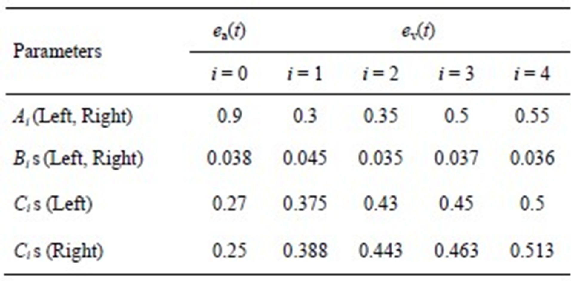
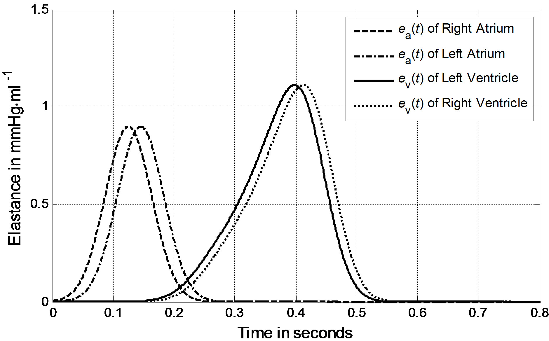
Figure 2. Activation functions for the left ventricle, right ventricle, left atrium and right atrium.
3) Blood Vessels The P-V relationships of systemic veins, vena cava and proximal arteries are not linear, i.e., the compliances of these vessels are not constant. The nonlinear blood vessel models are based on Lu and Clark [10], in which the compliances are described by the P-V relationship and the resistances of the vena cava and proximal arteries are nonlinear functions of blood volume.
Systemic veins. Vessels stiffen as their volume increases. The P-V relationship of systemic veins can be represented as follows,
 , (5)
, (5)
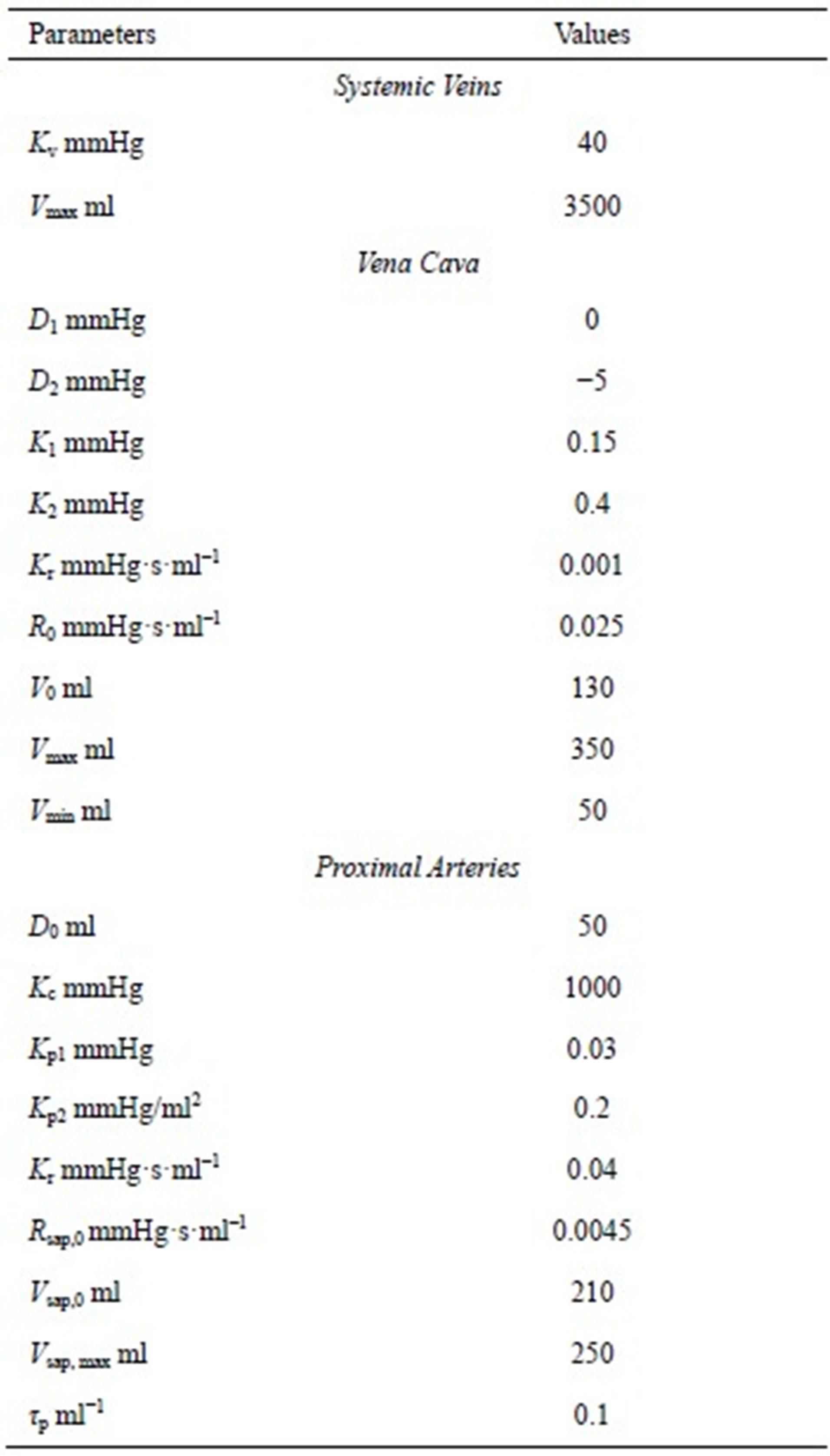
where Psv and Vsv are the pressure and volume of systemic veins, Kv is a scaling factor, and Vmax is the maximal volume of the systemic veins.
Vena cava. The P-V relationship of the vena cava is as follows,
 , (6)
, (6)
where Pvc and Vvc are the pressure and volume of the vena cava. V0 and Vmin are the unstressed and minimum volumes, respectively. The parameters K1, K2, D1 and D2 can be tuned to adapt the P-V relationship for the human venous system. The resistance of the vena cava is given as follows,
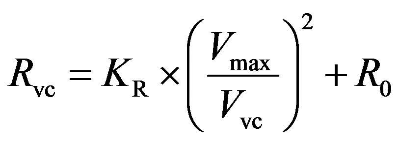 , (7)
, (7)
where KR is a scaling factor and R0 is the resistance offset.
Proximal arteries. As the compliance and resistance of proximal arteries are related to vasomotor tone, P-V curves of arteries must be different under fully activated or passive conditions. We describe the P-V relationship of proximal arteries as
Table 3. Parameters for nonlinear P-V curves and resistances in systemic veins, the vena cava and proximal arteries.
 , (8a)
 , (8b)
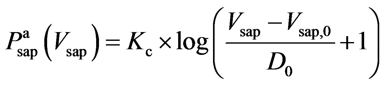
where  and
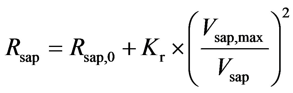
and  denote the fully activated and passive pressures of proximal arteries; Vsap is the volume; Vsap,0 is the minimal volume; Kc, Kp1 and Kp2 are scaling factors; D0 is a volume parameter; and τp is constant. The resistance is determined by Vsap as follows,
 , (9)
, (9)
where Rsap,0 is offset resistance, Vsap,max is the maximal volume, and Kr is a scaling factor. The all parameters used in this subsection are listed in Table 3.
2.2. Solution to the Cardiopulmonary Model
The cardiopulmonary model shown in Figure 1 can be solved numerically using an iteration scheme. An iteration loop is initialized from the onset of LV pressure rise at t = 0. All initial values for the volumes and flows are given in Appendix B. The simulated BP curves of one heart beat cycle for the left ventricle, left atrium and aortic artery are presented in Figure 3(a). The simulated BP curves for their counterparts in the pulmonary system are presented in Figure 3(b).
2.3. Definition of Heart Valve Closure Timing Intervals
According to hydrodynamics, the BP gradient across the heart valves causes the valves’ actions. Each valve opens or closes one time in a cardiac cycle depending on the differential pressure across the valve and thus contributes to the generation of heart sounds. The valve closure timings are thus defined by the relative pressures across the valves, as indicated by the arrows in Figure 3. The closure timings of the mitral valve, aortic valve, tricuspid valve and pulmonary valve are denoted as tm, ta, tt and tp, respectively. It is widely accepted that acoustic vibrations due to the closures of the mitral and tricuspid valves are major components of S1. Similarly, the closures of the aortic and pulmonary valves are the main contributors to S2. Therefore, heart sounds collected from the thorax surface can be used as timing markers of heart valve closures. Heart valve closure timings can thus be noninvasively monitored. Although the mechanism of heart sound generation is still in dispute, the timing correlations between heart sounds and heart valve closures have been widely accepted by researchers. Based on these facts, the timing intervals of any two valve closures are shown in Figure 4. For example, the timing interval between the mitral valve and tricuspid valve closures (TIMT) is calculated as the time interval between the mitral and tricuspid components of the first heart sound, i.e., Δtmt = tt – tm. Similarly, the other three timing intervals TIAP, TIMA and TIAM can be defined as Δtap = tp – ta, Δtma = ta – tm, and Δtam = tm – ta, respectively, as illustrated in Figure 4. The mitral valve closes at the onset of left ventricular contraction, while the aortic valve closes at the onset of left ventricular extension. Therefore, Δtma denotes the systolic time interval (STI) of a heart beat cycle, Δtam denotes the diastolic time interval (DTI), Δtap may be represented by the time split of the second heart sound, and Δtmt may be represented by the time split of the first heart sound. The objective of this paper is to investigate the relationships between LVSBP and heart valve closure timings, which can be non-invasively accessed by the timing intervals of heart sounds.
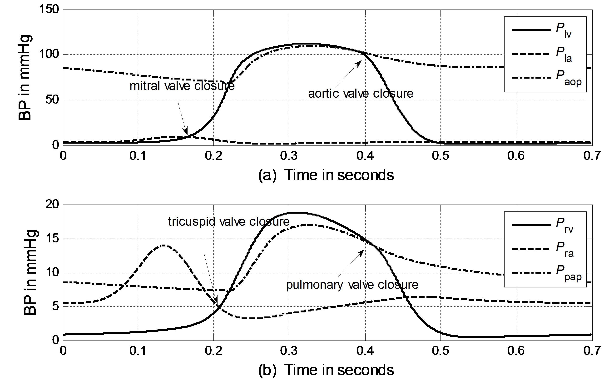
Figure 3. Simulated blood pressure of one heart cycle in the systemic and pulmonary circulations. (a) Systemic blood pressure; (b) Pulmonary blood pressure.
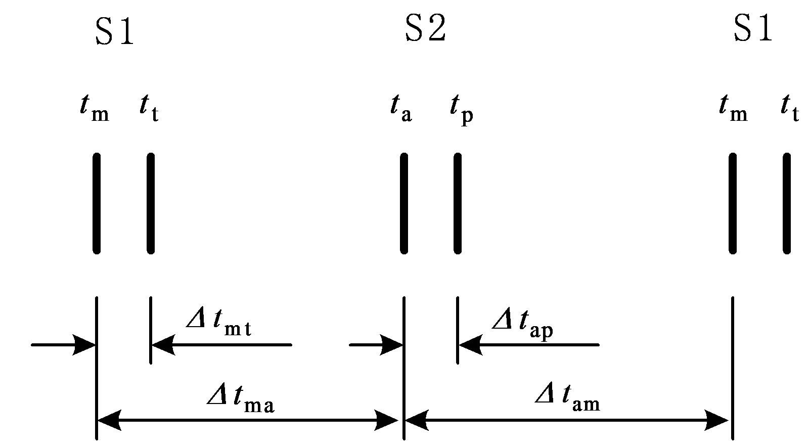
Figure 4. Valve closure timing intervals assessed using heart sounds. “S1” and “S2” denote the first and second heart sound, respectively.
2.4. Physiological Controls of the Model
1) Heart rate control Heart rate, characterized by Sunagawa as a three-dimensional response [15], is controlled by vagal and sympathetic neural activity. The human heart rate response to vagal and sympathetic input is further characterized by Lu and Clark [10]
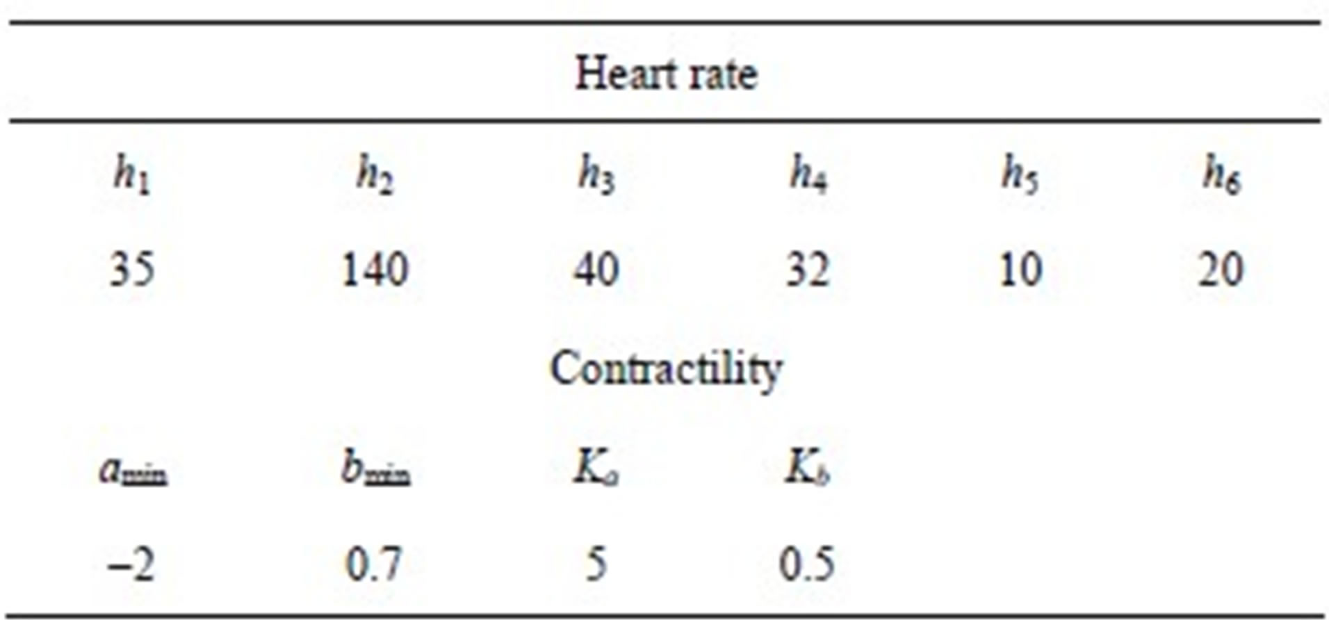
 , (10)
where h1 – h6 are constants that can be found in Table 4. FHrs and FHrv are normalized sympathetic and vagal discharge frequencies, respectively.
2) Ventricle contractility control From a physiological point of view, greater sympathetic tone increases myocardial elastance and shortens ventricular systole. Therefore, the ventricular activation function should be modified to describe the variation in the ventricular P-V relationship as a function of sympathetic efferent discharge frequency Fcon. A rising Fcon increases maximum elastance and shortens the systolic
Table 4. Parameter values for control of heart rate and contractility.
period. Eq.2 for the end-systolic P-V relationship then becomes
 , (11)
and the activation function ev(t) is rewritten as
 , (12)
where
 ,
,
 .
.
The constants amin and bmin represent the minimum values of the functions a and b. Ka and Kb are scaling parameters.
3) Vasomotor tone Proximal arteries. As mentioned in Section 2.1.3, arterial compliance and resistance are related to vasomotor tone, which is regulated by the normalized sympathetic frequency Fvaso. The P-V relationship of proximal arteries is characterized by
 , (13)
where  and
and  are given in (8a) and (8b). The resistance of proximal arteries becomes
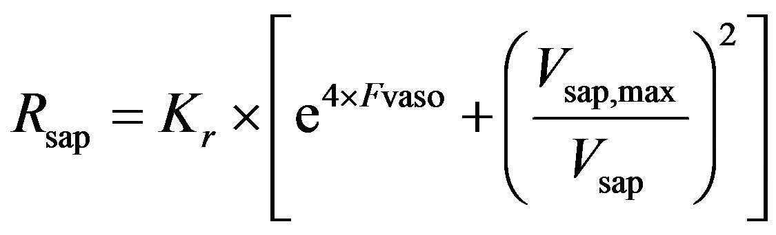 . (14)
As described in previous works [16,17], the compliance of the proximal aorta, Caop, decreases as blood pressure increases, indicating that diastolic pressure increases more slowly than systolic pressure. This phenomenon was also verified in the authors’ experiments. Caop is defined as a function of the sympathetic frequency Fvaso,
 . (15)
3. SIMULATION RESULTS
3.1. Blood Pressure and Heart Rate in Response to Exercise
In the simulation, it is assumed that a virtual subject follows a two-phase physiological routine. The total simulation time for the two-phase routine is 300 seconds. The virtual subject begins in a resting state and is then asked to exercise in the first phase for the first 100 seconds and stop exercising to recover in the second phase for the next 200 seconds. In the resting state, the sympathetic and vagal nerves contribute to heart rate control in equal degrees. In the simulation, the normalized sympathetic (FHrs, Fcon, Fvaso) and vagal (FHrv) frequencies are initialized at 0.5. During exercise, sympathetic (Fcon, FHrv, Fvaso) frequencies become dominant; meanwhile, vagal (FHrv)
frequency decreases, as shown in Figure 5 for the first 100 seconds. Once the subject stops exercising after 100 seconds, sympathetic (Fcon, FHrs, Fvaso) frequencies immediately begin to decrease, and vagal (FHrv) frequency begins to increase. Finally, all frequencies converge at 0.5. As we expected, the subject’s heart rate and LVSBP increase during the first phase and decrease during the second phase. Simulation results based on this platform are given in Figure 6 and show that the heart rate begins at 76 beats per min, increases to 107 beats per min, and finally returns to 76 beats per min. LVSBP starts at 120 mmHg and increases to 160 mmHg at the end of the exercise period. LVSBP returns to 120 mmHg as the subject recovers to the resting state.
3.2. Timing Intervals in Response to Exercise
Using the definitions of timing intervals given in Section 2.3, the responses of Δtma, Δtam, Δtap and Δtmt to LVSBP in the two-phase routine can be calculated, as illustrated in Figure 7. Solid lines represent the relationships in the exercising phase, and dashed lines represent the relationships in the recovery phase. The fact that the solid and dashed lines nearly overlap means that the two-phase physiological routine is reversible. The subject begins from a resting physiological condition, reaches a maximum load at the 100th second, and comes back to the original resting state at the end of the simulation following a reversible physiological routine. It can be seen in Figure 7 that Δtma, Δtam and Δtap have strong negative relationships with LVSBP in both phases, while Δtmt has a slightly negative relationship. These relationships imply that hemodynamic variations in the left ventricle can be reflected in heart valve closure timing intervals. These intervals tend to decrease with increasing LVSBP.
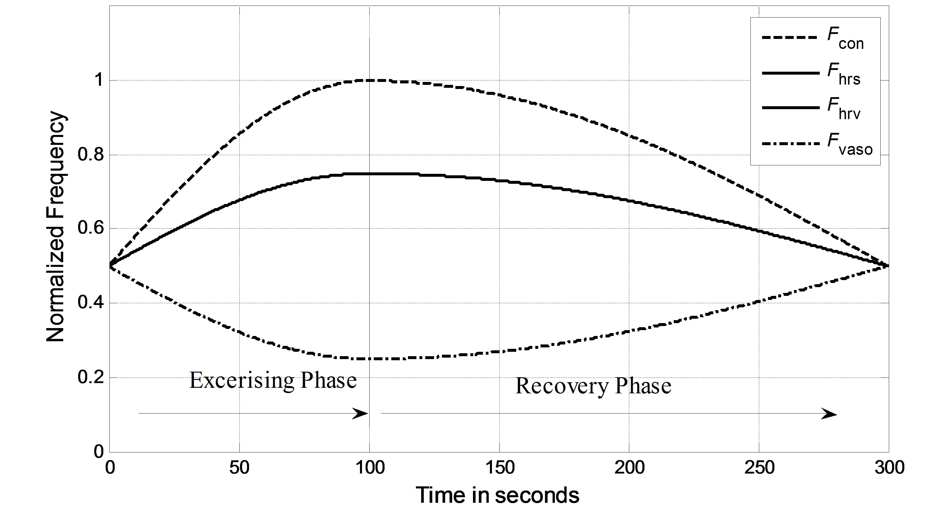
Figure 5. Normalized vagal and sympathetic frequencies in the two-phase routine.

Figure 6. Simulated heart rate and LVSBP in the two-phase exercise routine. (a) LVSBP; (b) Heart rate.

Figure 7. Simulated relationships between Δtma, Δtmt, Δtap, Δtam and LVSBP.
4. EXPERIMENTAL VERIFICATIONS
4.1. Data Collection
Six young male subjects participated in the experiments, and they had a mean age of 27 ± 3 years (means ± SE). The experiment protocol was approved by the local ethics committee. All of the subjects gave their consent to participate in the experiments. They were asked to stay at rest for 10 minutes before exercise. This resting state may be taken as a baseline for blood pressure. They were asked to perform a step-climbing exercise for 100 steps and lie on their backs on an examination table immediately afterwards. Heart sounds and ECG signals were simultaneously recorded at a sampling frequency of 2 KHz (Biopac MP150, USA), for which the heart sound microphone sensor was placed in an optimal position on the thorax to distinguish heart sound components. Blood pressure was measured immediately after each signal recording by a standard electronic oscillometric meter on the upper left arm (HEM-7200, OMRON, Japan). The signal recording lasted 300 seconds (5 minutes) so that the subjects had almost recovered to the resting state. Blood pressure values at any other time may be estimated using interpolation.
4.2. Data Analysis
The signals were contaminated by breathing sounds at the beginning of the recordings. One may use our previously developed noise reduction technique to improve signal quality [18,19]. Although researchers have not come to a consensus on the mechanism of heart sound generation [20,21], the fact that the timings of the heart sounds reflect the timings of heart valve closures has been widely accepted. To the authors’ knowledge, no fully developed automatic scheme is available to extract the time intervals Δtma, Δtam, Δtap and Δtmt from heart sound signals. In this study, the authors adopted a time-frequency technique with the ECG signal as a reference to detect the timing intervals. Each heart sound signal was first segmented into cycles with the assistance of simultaneously sampled ECG R-waves. Then, continuous wavelet analysis, as illustrated in [22], was used to extract the intervals between peaks. Each cycle of a heart sound signal contains a group of Δtma, Δtam, Δtap and Δtmt. Hundreds of groups of intervals were thus determined from a 300-second recording. The scatter plots of the intervals with respect to LVSBP for one subject are depicted in Figure 8, showing that all of the intervals have negative relationships with LVSBP. From visual observation, Δtma, Δtam, Δtap have much stronger negative relationships to LVSBP, while the LVSBP relationship with Δtmt is much less negative. The experimental results for Δtma, Δtam and Δtap are very close to the simulation results. The result for Δtmt agrees with that of the simulation, but the experimental Δtmt shows a slightly stronger negative relationship than that of the simulation.
To further demonstrate the negative relationships between the intervals and LVSBP for the 6 subjects, the relationships were fitted to first-order equations based on the least squares criteriaΔt = Slope∙PLVSBP+ Offset. (16)
The slopes and offsets are listed in Table 5. The slopes and offsets vary among the subjects. It can be seen that Δtma, Δtam and Δtap have strong negative relationships with LVSBP, while Δtmt has a slightly negative relationship.

Figure 8. Experimental relationships between Δtma, Δtmt, Δtap, Δtam for a subject.
Table 5. Slopes and offsets of the best-fit lines for the 6 subjects.

5. DISCUSSION
From the physiological point of view, heart rate and cardiac muscle contractility will increase rapidly during exercise in the first phase, causing the systolic and diastolic time intervals to become shorter. These phenomena are reflected in heart sounds, i.e., Δtma and Δtam become shorter than in the resting state. Additionally, the increasing cardiac muscle contractility of the left ventricle leads to a shorter ejection period, causing aortic valve closure to shift to an earlier time. However, pulmonary valve closure shifts to an even earlier time. Therefore, the interval Δtap decreases in the final presentation. Both experimental and simulation results show that Δtma, Δtap and Δtam have strong negative relationships to LVSBP.
However, the results for Δtmt were less consistent. Simulations showed that Δtmt had a very small negative change with respect to LVSBP, while the experimental results showed a slightly stronger negative relationship. There are two possible factors that may have caused this result. 1) The parameter Δtmt was extracted with peak location using time-frequency analysis; location errors were unavailable; 2) The values of the resistors Rm and Rt in the analog circuit shown in Figure 1 can affect the pressure timing across the mitral and tricuspid valves. Improper values for the resistors may cause the timings to be less accurate.
It may be concluded based on both simulations and experiments that Δtma, Δtam, Δtap are more sensitive to LVSBP and that Δtmt is less sensitive to LVSBP. These relationships may have potential applications in continuously monitoring LVSBP with a high time resolution of one heartbeat. It is possible to monitor relative variations in LVSBP without any calibration if heart sound signals can be collected during regular medical checkups. Hemodynamic disorders may be found in earlier stages of progression after performing long-term monitoring of the intervals.
In addition, another phenomenon, shown in Figure 8, is that the intervals vary greatly locally. This is believed to be caused by respiration. The respiration modulation of heart sound morphology was also observed by previous researchers, as illustrated in [23,24].
6. CONCLUSIONS
A modified mathematical model of the cardiopulmonary system was proposed as a platform to study the relationships between heart valve closure timing intervals and LVSBP, in which a vagal-sympathetic mechanism was introduced to control heart rate and ventricle contractibility. Four intervals, Δtma, Δtmt, Δtap and Δtam, based on the differential pressures across the valves, were defined to describe the valve closure timing intervals.
Using this platform, it was found that the hemodynamics vary as heart rate and ventricle contractibility increase. Simulation results show that Δtma, Δtap and Δtam bear strong negative correlations with LVSBP and that Δtmt has slight negative relation. To further validate these relationships, 6 subjects participated in a two-phase experiment. The four intervals were extracted from heart sound signals collected from the surface of the thorax. The experimental results agree with those obtained from simulations. This study helps in the understanding of the hemodynamic response to various physiological conditions. The method described may have potential applications in the continuous and non-invasive monitoring of heart chamber hemodynamics based on the heart sound features.
7. ACKNOWLEDGEMENTS
This work was supported, in part, by the Fundamental Research Funds for the Central Universities under grant DUT12JB07, DUT12JR03 and the National Natural Science Foundation of China under grant 81000643.
REFERENCES
- Durand, L.G. and Pibarot, P. (1995) Digital signal processing of the phonocardiogram: Review of the most recent advancements. Critical Reviews in Biomedical Engineering, 23, 163-219. doi:10.1615/CritRevBiomedEng.v23.i3-4.10
- Hamada, M., Hiwada, K. and Kokubu, T. (1990) Clinical significance of systolic time intervals in hypertensive patients. European Heart Journal, 11, 105-113. doi:10.1093/eurheartj/11.suppl_I.105
- Zhang, X.Y., MacPherson, E. and Zhang, Y.T. (2008) Relations between the timing of the second heart sound and aortic blood pressure. IEEE Transactions on Biomedical Engineering, 55, 1291-1297. doi:10.1109/TBME.2007.912422
- Lewis, R.P., Rittogers, S.E., Froester, W.F. and Boudoulas, H. (1977) A critical review of the systolic time intervals. Circulation, 56, 146-158. doi:10.1161/01.CIR.56.2.146
- Weissler, A.M., Harris, W.S. and Schoenfeld, C.D. (1968) Systolic time intervals in heart failure in man. Circulation, 37, 149-159. doi:10.1161/01.CIR.37.2.149
- Chen, D., Pibarot, P., Honos, G. and Durand, L.G. (1996) Estimation of pulmonary artery pressure by spectral analysis of the second heart sound. American Journal of Cardiology, 78, 785-789. doi:10.1016/S0002-9149(96)00422-5
- Dennis, A., Michaels, A.D., Arand, P. and Ventura, D. (2010) Noninvasive diagnosis of pulmonary hypertension using heart sound analysis. Computers in Biology and Medicine, 40, 758-764. doi:10.1016/j.compbiomed.2010.07.003
- Matsuda, T., Kumahara, H., Obara, S., Kiyonaga, A., Shindo, M. and Tanaka, H. (2008) The first heart sound immediately after exercise stress. International Journal of Sport and Health Science, 6, 213-218. doi:10.5432/ijshs.IJSHS20080326
- Tranulis, C., Durand, L.G., Senhadji, L. and Pibarot, P. (2002) Estimation of pulmonary arterial pressure by a neural network analysis using features based on timefrequency representations of the second heart sound. Medical and Biological Engineering and Computing, 40, 205-212. doi:10.1007/BF02348126
- Lu, K., Clark, J.W. and Ghorbel, F.H. (2001) A human cardiopulmonary system model applied to the analysis of the Valsalva maneuver. American Journal of Physiology—Heart and Circulatory Physiology, 281, H2661- H2679.
- Olansen, J.B., Clark, J.W. and Khoury, D. (2000) A closed-loop model of the canine cardiovascular system that includes ventricular interaction. Computers and Biomedical Research, 33, 260-295. doi:10.1006/cbmr.2000.1543
- Ursino, M. (1998) Interaction between carotid baroregulation and the pulsating heart: A mathematical model. American Journal of Physiology—Heart and Circulatory Physiology, 275, H1733-H1747.
- Chung, D., Niranjan, S., Clark, J.W., Bidami, A., Johnston, W.E., Zwischenberger, J.B. and Traber, D.L. (1997) A dynamic model of ventricular interaction and pericardial influence. American Journal of Physiology—Heart and Circulatory Physiology, 6, H2942-H2962.
- Braunwald, E., Fishman, A.P. and Cournand, A. (1956) Time relationship of dynamic events in the cardiac chambers, pulmonary artery and aorta in man. Circulation Research, 4, 100-107. doi:10.1161/01.RES.4.1.100
- Sunagawa, K., Kawada, T. and Nakahara, T. (1998) Dynamic nonlinear vago-sympathetic interaction regulating heart rate. Heart Vessels, 13, 157-174. doi:10.1007/BF01745040
- Loannou, C.V., Stergiopulos, N. and Katsamouris, A.N. (2003) Hemodynamics induced after Acute Reduction of Proximal Thoracic Aorta Compliance. European Journal of Vascular and Endovascular Surgery, 26, 195-204. doi:10.1053/ejvs.2002.1917
- Takeshi, O., Seiji, M. and Motoyuki, L. (2008) Systemic arterial compliance, systemic vascular resistance, and effective arterial elastance during exercise in endurancetrained men. American Journal of Physiology—Heart and Circulatory Physiology, 295, R228-R235.
- Tang, H., Li, T., Park, Y. and Qiu, T. (2010) Separation of heart sound signal from noise in joint cycle frequency-time-frequency domains based on fuzzy detection. IEEE Transactions on Biomedical Engineering, 57, 2438- 2447. doi:10.1109/TBME.2010.2051225
- Tang, H., Li, T. and Qiu, T. (2010) Noise and disturbance reduction for heart sounds in the cycle frequency domain based on non-linear time scaling. IEEE Transactions on Biomedical Engineering, 57, 325-333. doi:10.1109/TBME.2009.2028693
- Heintzen, P. (1961) The genesis of the normally split first heart sound. American Heart Journal, 62, 332-343. doi:10.1016/0002-8703(61)90399-4
- Waider, W. and Craige, E. (1975) First heart sound and ejection sounds: Echocardiographic and phonocardiographic correlation with valvular events. American Journal of Cardiology, 35, 346-356. doi:10.1016/0002-9149(75)90026-0
- Debbal, S.M. and Ereksi-Reuig, F. (2008) Computerized heart sounds analysis. Computers in Biology and Medicine, 38, 263-280. doi:10.1016/j.compbiomed.2007.09.006
- Amit, G., Shukha, K., Gavriely, N. and Intrator, N. (2009) Respiratory modulation of heart sound morphology. American Journal of Physiology—Heart and Circulatory Physiology, 296, H796-H805. doi:10.1152/ajpheart.00806.2008
- Castle, R.F. and Jones, K.L. (1961) The mechanism of respiratory variation in splitting of the second heart sound. Circulation, 24, 180-184. doi:10.1161/01.CIR.24.2.180
APPENDIX A: PARAMETERS OF THE CARDIOVASCULAR MODEL
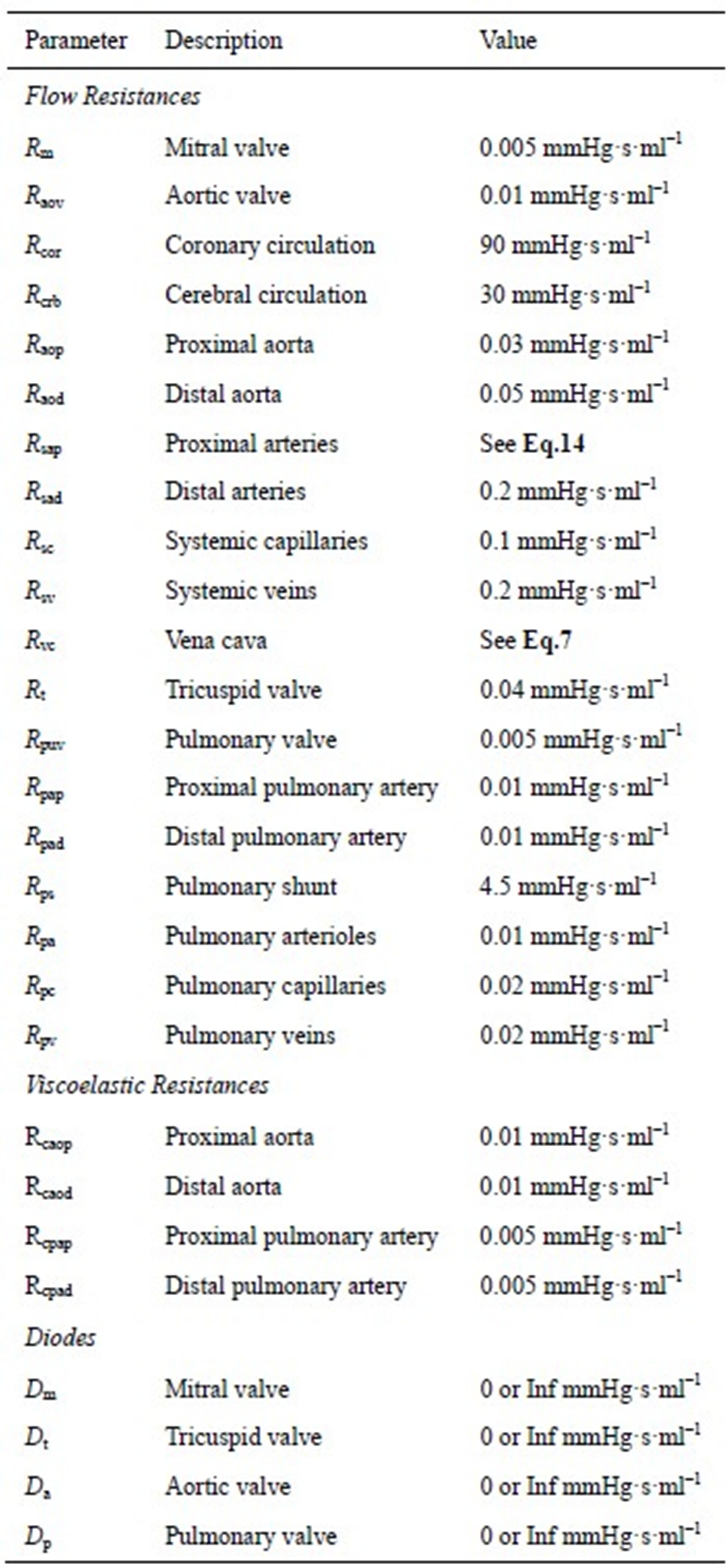
The model of the cardiovascular system presented in this article was simulated using the parameter values listed in Tables A1-A3. Because the hemodynamic parameters vary among human individuals, the values of the resistors, diodes, capacitors and inductors in this appendix reflect those of a typical human being and were obtained based on reasonable blood pressure values at reference knots in the circuit.
Table A1. Resistors and diodes of the cardiovascular model.
APPENDIX B: INITIAL CONDITIONS OF THE CARDIOVASCULAR MODEL
Initial conditions of the model include heart chamber and vascular volume, and systemic and pulmonary aorta flow, corresponding to the charges of the capacitors and the currents of the inductors. The initial values were obtained based on considerations of both reasonable blood distributions and total blood volume. A feasible set of parameters are listed in Table B1.
Table A2. Inductors of the cardiovascular model.
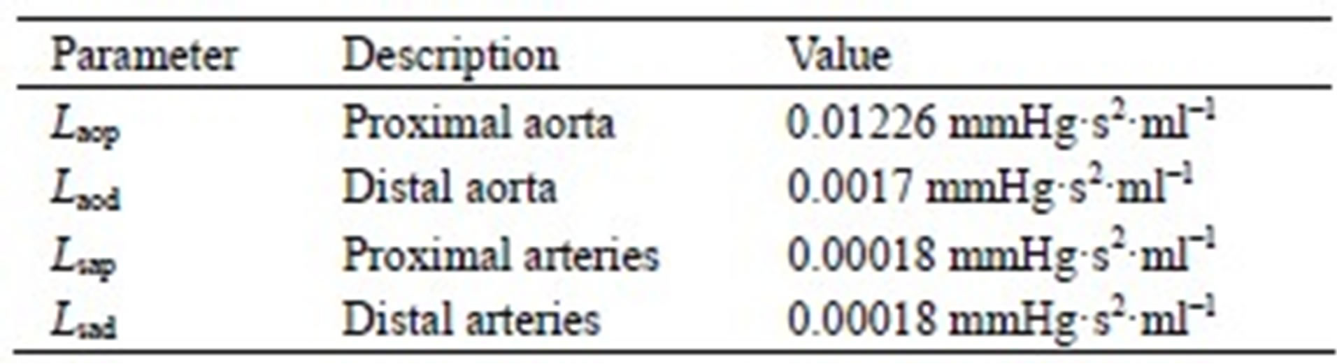
Table A3. Capacitors of the cardiovascular model.

Table B1. Compliances of the cardiovascular model.
