Journal of Geographic Information System
Vol. 5 No. 1 (2013) , Article ID: 27927 , 9 pages DOI:10.4236/jgis.2013.51009
The Multiresolution Image Format
1Institute of Geography, University of Pécs, Pécs, Hungary
2Doctoral School of Earth Sciences, University of Pécs, Pécs, Hungary
Email: titusz@gamma.ttk.pte.hu, halmaia@gamma.ttk.pte.hu
Received September 25, 2012; revised October 28, 2012; accepted November 29, 2012
Keywords: Multiresolution; Image Storing; Raster; GIS
ABSTRACT
In this paper we present a new method and file format which allows to create, store and manipulate multiresolution raster images. “Classic” raster images are built up by rasters (pixels) where in the same image each raster (pixel) has the same size. Multiresolution raster image (mri) are unlike the “classic” raster images. An mri file is a regular text file, conformed xml 1.0 standard and allows: 1) to store raster based images with different resolution in the same file and in the same time (i.e., allows to contain rasters with different size in the same image); 2) to export easily any part of the image as a separate raster image and to import an image as a part of a raster; 3) to define geographical reference for a raster image and use this image as a raster based GIS model; 4) to perform computations (i.e., image manipulation) on the content of the file. It is an important characteristic of the mri format that mathematical operations could be performed always in the same resolution as the current resolution of the given part of the image. To confirm this statement we present how to perform a convolution on an mri file.
1. Introduction
Raster based data storage is a common way in the image processing and manipulating. It is widely used by spatial informatics systems too, as “raster based data model”.
There are many raster based file formats nowadays, but at least in one point all of them are very similar to each other: the image contained by the file, has only one resolution on the entire image. This means that number of pixels of the image unambiguously can be computed knowing dimensions of this image (columns and rows). When the hardware used for displaying this image also known, the actual resolution can be defined as DPI.
Hence, because the resolution in the separate parts of an image can not be changed, there is no way to store image data with different resolution in the same image. In case where two or more different resolution raster image of the same object is to be used, separate images with the adequate resolution has to be created—one file for each resolution, or at least one layer for each resolution.
An example should help to expose the problem.
Let there be a raster based map (spatial model) that contains data of a valley and it has a resolution of 10 × 10 meters and in the mid-line of this valley a watercourse. The aim is to survey its surround in more detailed than the valley itself, e.g. in 1 × 1 meter resolution. There are only two options to store results in the same raster file.
• The first choice is to reduce the resolution of the more detailed parts of the image, to fit data to low resolution parts of map. This makes the detailed surveying itself pointless.
• The other way is to improve the resolution of the low resolution parts to fit to those more detailed areas.
In latter case, the low resolution rasters will be resampled and new rasters will be created, using an adequate interpolation method. This is the commonly used method, for it gives the possibility to use the results of surveying and the previously existing image data in the same time and in the same file. Disadvantage of this solution is the need for more memory, more CPU-time and more storage capacity.
Our research gives a possible solution for this question and for similar cases too.
Peucker et al. (1978) [1] recognized the same problem in the field of the digital terrain representation. Their famous article “The Triangulated Irregular Network” gives a good solution to store and represent non-equally spaced vector (elevation) data. But there was no significant precedent found in scientific papers on multiresolution image (raster-based) format, presented in this paper.
2. Multiresolution Image Container File Format
Multiresolution image format (mri)1 is an ASCII XML file, conformed to xml version 1.0 (see detailed technical description in Bray et al. 2008) [2]. We chose the xml standard, because it is an open, crossplatform format, and also widely used in the field of geomatics, in most cases to represent vector based data (Antoniou & Tsoulos 2006) [3]. The mri format allows to create and use multiresolution parts in the same file and in the same time (see Figures 1 and 2). It also allows taking mathematical operations (image processing) on data with different resolutions, handling different resolutions rasters (pixels) as a uniform array.
Essential characteristics of this format is, that each sub-resolution can easily be exported as a separate image and also simple to attach a more detailed dataset to any raster of the image.
The mri format allows to store information as raster based GIS data with the adequate spatial references or simple image data without any spatial references. This means, that the same dataset can be handled as a simple raster image or if it is needed, as a raster based, georeferenced GIS model.
Mri is a hierarchically structured format: each resolution is a resolution-level and each resolution-level might have a sub-resolution. Iteration is allowed, hence theoretically it is not limited the number of sub-resolutions. The base thought is, that a raster image can be defined not only as a matrix, but as a hierarchically structured vectors too, when each line of a raster image is a vector and any vector can be linked to any other vector using a properly defined pointer in the file. As xml is itself a hierarchical language with links and pointers, mri format
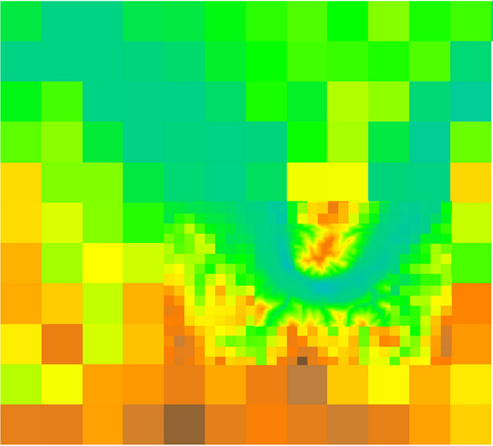
Figure 1. An example for multiresolution image. The river Danube in Hungary, north from Budapest. This is not a real model, only an illustration, made by Libre Office Draw, based on three different resolution DEM: 1200 m/raster, 300 m/raster and 30 m/raster.
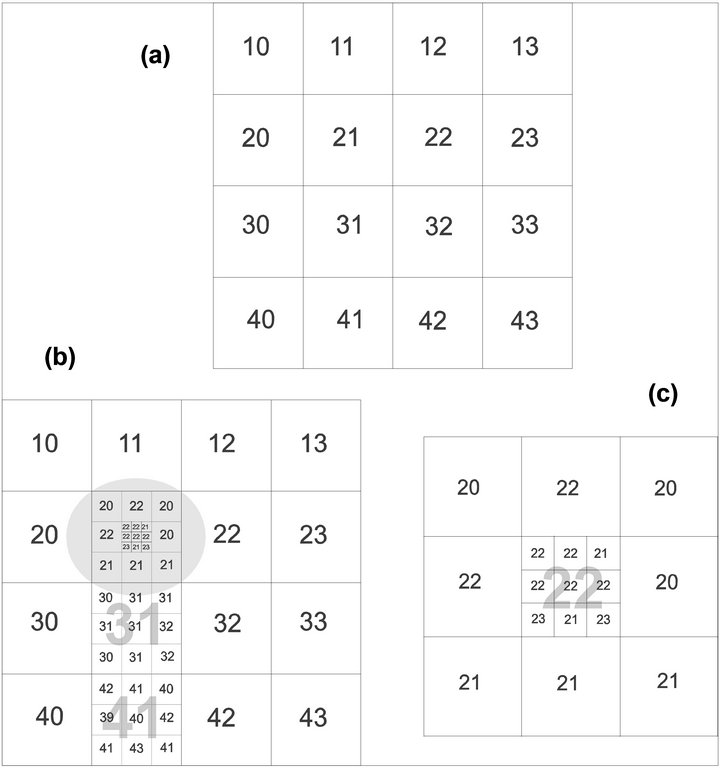
Figure 2. (a) A regular raster image; (b) A multiresolution image. Three raster has a sub-resolution and one raster has two sub-resolution (grey background). (c) Raster with grey background of Figure 2(b) in detail. This part of the original image might be handled as a separate raster image if necessary.
were defined as an regular text file conformed to xml standard.
The base resolution (highest-level resolution) of an image named as resolution 0 (zero). Resolution 0 is a quadratic-shape raster image, where there are M columns × N rows and each raster (cell) have to contain exactly one attribute data or at least a NO_DATA notes.
Any raster of Resolution 0 may have a sub-resolution, named as resolution 1. This means that there is an attribute dataset attached to the given raster of Resolution 0, which represents the inner part of this raster. Resolution 1 characterized by its size as m columns × n rows. Similarly to resolution 0, each raster have to contain exactly one attribute data or at least a NO_DATA notes.
Resolution 1 may also have a sub-resolution, named as Resolution 2, and so on.
Each raster can only have the same sub-resolution on the same resolution-level. This means, that when a raster exists on resolution-level 0 with sub-resolution resolution 1, other raster on resolution-level 0, can only have the same resolution 1. For example, if a raster of resolution-level resolution 0 have a sub-resolution 40 × 40 (resolution 1), then any other raster of resolution 0 can only have a sub-resolution 40 × 40.
Please note that resolution of resolution-levels can differs, so it is possible to define different resolution for each resolution-level separately.
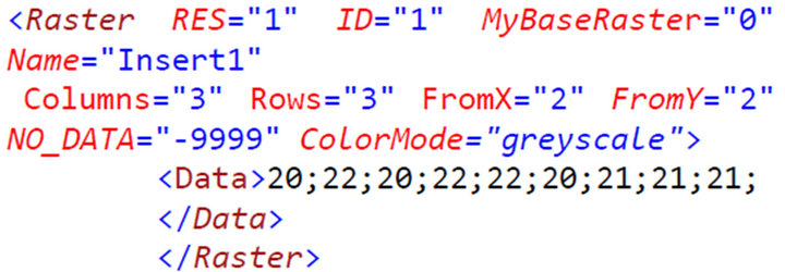
Now, below it is an mri file, that contains data of raster image b of Figure 2. on page 3 and its explanation.
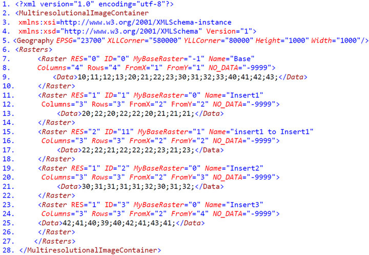
• Lines 1 to 4:
General xml notes.
• Line 5:
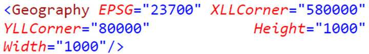
Geographical metadata. If exists, data follows in the file, have to be interpreted as a raster based GIS model. If not exists (i.e., the tag is not in the file), data has to be interpreted as a raster image, without any spatial reference.
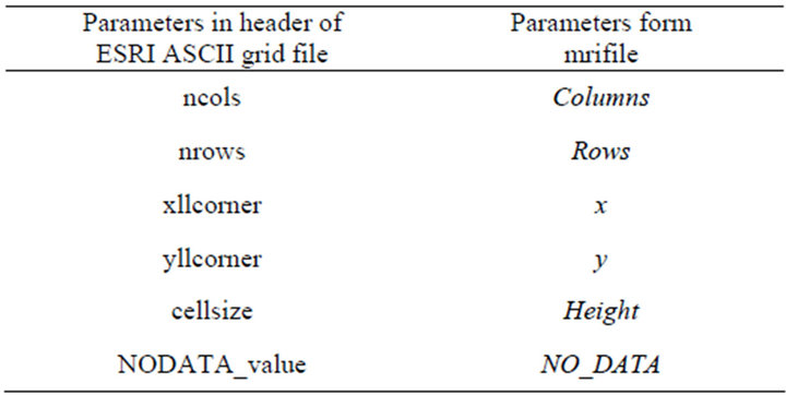
Geographical metadata is very similar to the header of a standard ESRI ASCII raster file, hence the conversion from ESRI ASCII to mri and vice versa becomes a simple process.
EPSG—EPSG code of used projection system.
XLLCorner—X coordinate of the lower left corner of the image.
YLLCorner—Y coordinate of the lower left corner of the image.
Height2—The real height of a raster, in units defined by the used projection system.
Width—The real width of a raster, in units defined by the projection system in use.
• Line 6:
Rasters—Signs the begin of all resolution’s raster attribute data. It always has to be ended by /Rasters at the end of definition of all raster attribute data of all resolutions (see: Line 27).
• Line 7 - 10:
Definition of a resolution.
Raster—Beginning of definition of a resolution. Has to be closed by/Raster (see: Line 10).
RES—Level of resolution. Always has to be followed by an integer as parameter. An mri type raster image always has to contain a base level resolution (named as “resolution zero”) and its parameter is 0 (zero).
ID—Identifier of the attribute data series contained by the given Raster. The parameter is an integer, defined by the user or the creator of the file.
MyBaseRaster—Identifier of the parent resolution level. In case where RES = 0, it has a parameter—1 (because resolution zero has no parent resolution). In any other case the parameter is equal to the parameter of RES of the parent resolution level.
Name—Name of the resolution, given by the user. Free formed character string.
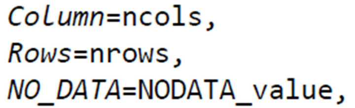
Columns—Number of the columns.
Rows—Number of the rows.
FromX—Denotes the number of the column in which the parent raster of the given resolution can be found. If value of RES is zero, FromX must be 1.
FromY—Denotes the number of the row in which the parent raster of the given resolution is to be found. If value of RES is zero, FromY must be 1.
NO_DATA—Integer, value of the raster cells with no data.
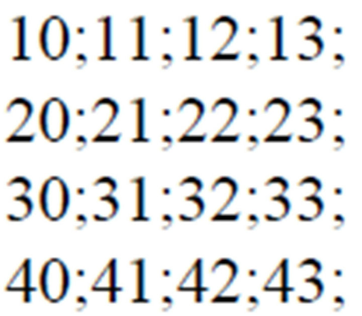
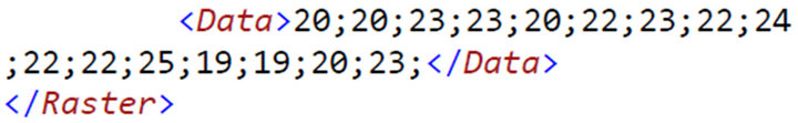
Data—Attribute data series. Each number shows the attribute data of a raster. Numbers are written one after the other, separated by a semicolon. The last character has to be a semicolon, white spaces are ignored. The first number is the attribute data of the upper left raster and the last number is the same of the lower right raster. Attribute data read from left to right, draws the matrix row by row from left to right, top to bottom.
All data structures are white-space independent, hence 10;11;12;13;20;21;22;23;30;31;32;33;40;41;42;43;will be the same as
• Line 11 - 14:
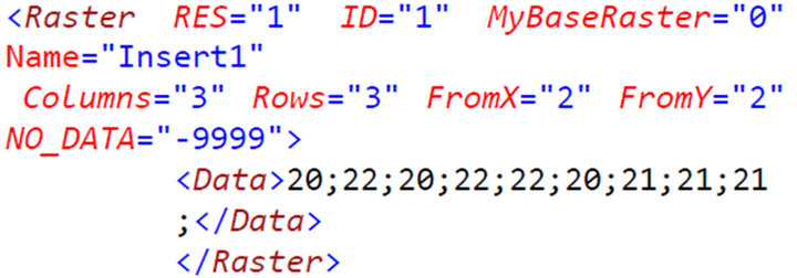
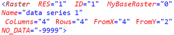
Definition of a sub-resolution. The structure is the same as shown in lines 7 - 10. Now RES is equal to 1 which shows that it is a first level sub-resolution, and ID and Name are also different. Value of MyBaseRaster (0) refers to Resolution 0, as parent resolution. As it can be read from values of Columns and Rows, it is a 3 × 3 matrix, a sub-matrix (sub-resolution) of the raster which has coordinates X = 2; Y = 2 of Resolution zero.
• Line 15 - 18:
• Second sub-resolution level, sub-resolution of Resolution 1. Interpretation is the same as above.
• Line 19 - 22:
First level sub-resolution of the raster in resolution zero, where X = 2; Y = 3.
• Line 23 - 26:
First level sub-resolution of the raster in resolution zero, where X = 2; Y = 4.
• Line 27:
Closing tag of definition for all resolutions.
• Line 28:
End of file tag.
2.1. Data Exchange
Mri format allows to exchange attribute data between other files using a simple text editor. It also allows to handle a sub-resolution as a separate image in a separate file, or to insert a content of an image in the mri file as a sub-resolution.
2.1.1. Data Extract from an Mri File
Let us aim to create a new, raster based GIS file using a sub-resolution level 1, where ID = 1 (it is defined in lines 11 - 15 in the example). In this case the operations are as follows.
• Step 1 Copying of lines 11 - 14 to a new, empty file.
• Step 2 Using informations of mri file contained in Geography tag (line 5 in the example) and values of parameters Columns, Rows, FromX, FromY and NO_DATA of sub-resolution, has to create an ESRI ASCII type header for the new file.
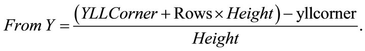
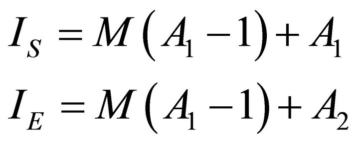
If XLLCorner—Lx
YLLCorner—Ly
Height—h Width—w From X—Sx
From Y—Sy
then
 (1)
(1)
when x = X is one of the coordinates of the lower left corner in the new file.
Furthetmore
 (2)
(2)
when y = Y is the other coordinate of the lower left corner in the new file. Using the actual values of the example on the page 5 , x = 581,000 and y = 81,000.
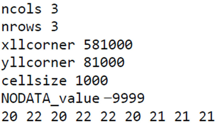
• Step 3 The creating of the attribute data for ESRI ASCII grid by using data in Data tag of mri file. Since the mri file uses semicolons to separate data, and ESRI ASCII grid uses spaces, hence required to change semicolons to spaces, but other data conversion (or structural conversion) is not necessary.

The result is an ESRI ASCII grid:
2.1.2. Data Insert into an Mri File
Goal-matrix is the matrix the data series has to be inserted, while the source-matrix is the source of the data series. In the actual sample the goal-matrix is the file presented on page 5, and the source-matrix is as follows:
ncols 4
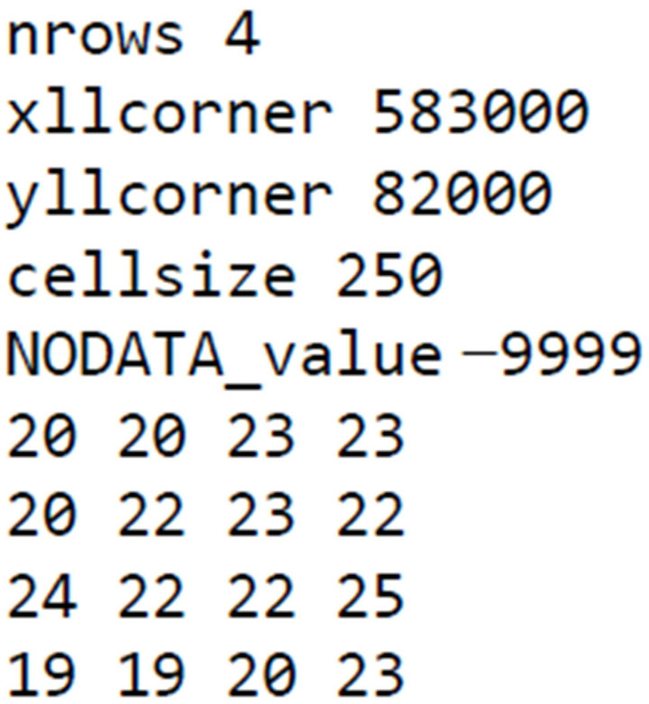
To create a sub-resolution using source dataset, there has to be Columns, Rows, FromX, FromY and Nodata defined.
Now,

Data series itself remains the same, but numbers ha convolution matrix which is no larger than 2m + 1 × 2n + 1 as to be separated by a semicolon and the last character also has to be a semicolon.
Using resultant values, sub-resolution can be defined as follows:
Copying this text into the original mri file (page 5 .), the result will be a new sub-resolution of raster X = 4, Y = 2 in resolution level RES 0.
3. Mathematical Operations—Convolving a Multiresolution Image
Mri format allows to perform mathematical operations on image. In this paper convolution will only be presented, because it is a complex and general method in the field of raster image processing. It is an important characteristic of mri format, that results of a convolution will be the same resolution as the original matrix had.
The following example presents a way to apply a convolution matrix to determine average of attribute data of cells.
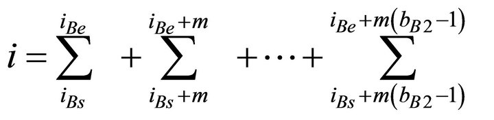
Equations presented has one significant limitation: a convolution matrix that is not larger than 2m + 1 × 2n + 1 can only be used. However it is easily can be overpassed using equations of Part 3.2 .
3.1. Denominations
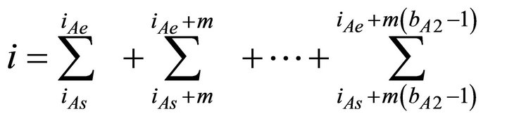
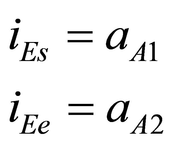
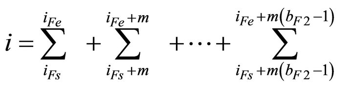
For example, when convolution matrix is on the bottom right corner of the sub-resolution, section A, B, E and F has to be considered.
3.2. General Convolution for Resolution 0
The following equations show how to convolve a regular (non-multiresolution) images, when image is M × N and convolving matrix is J × K (see Figure 3).
 (3)
(3)
 (4)
(4)
 (5)
(5)
3.3. Convolution for Sub-Resolution
Convolution of multiresolution parts of an image differs from the convolution of a simple raster image. Our first task is to define all the possible areas (see Figure 4). The second step is to give the equations for each section (see parts from 3.3.2 to 3.3.11).
The equation of an area describes how to compute the required result. These equations are built up from sepa-
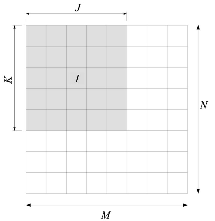
Figure 3. A raster image and a convolution matrix. Cells with gray background are in the convolution matrix while I is the center of this matrix. Result of convolution will be written in this cell. Convolution matrix has dimensions I columns × K rows. Dimensions of the raster image itself are M columns × N rows.

Figure 4. Nine sections of computation. Section A is on the sub-resolution, sections B to I are on adjacent cells (see equaations).
rate vectors. Each vector is a unique line (cells one after the other from left to right) in the given section.
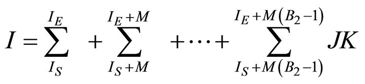
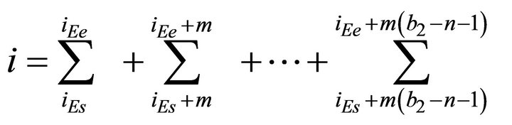
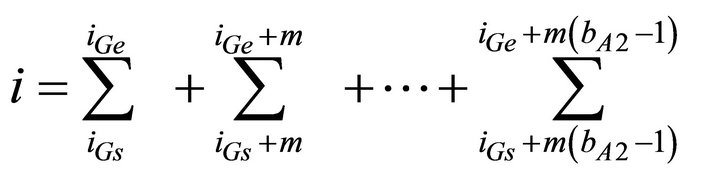
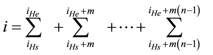
Let us assume that the aim is to compute the average of attribute data of cells under the convolution matrix. Then each equation will be the sum of a vector and the sum of all vectors divided by the number of cells of convolution matrix (j × k, see Figure 5) giving the searched result.
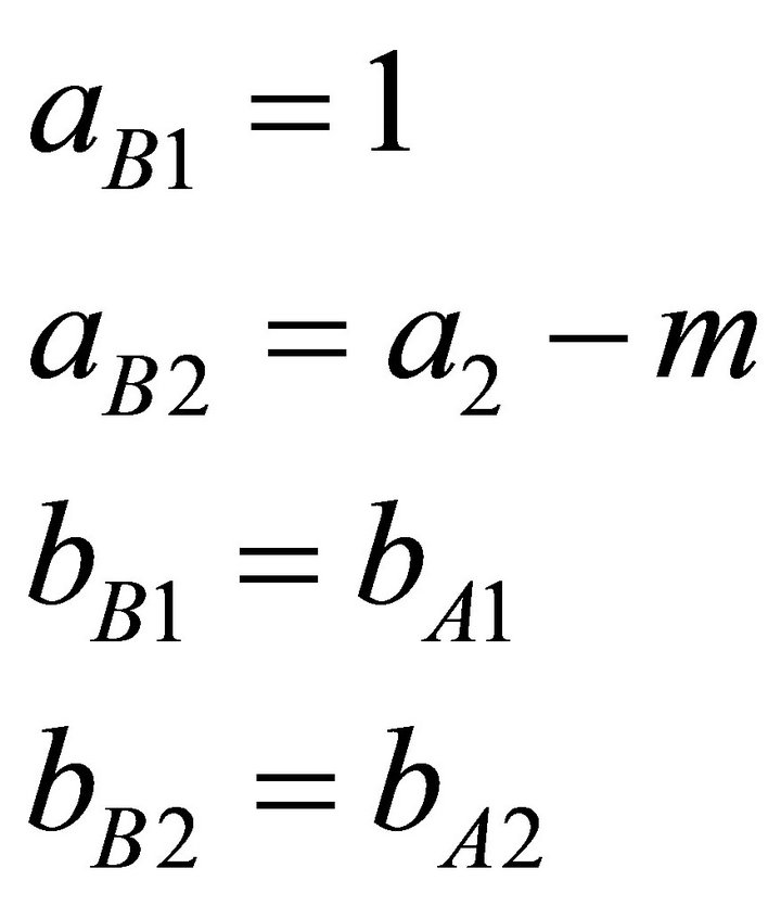
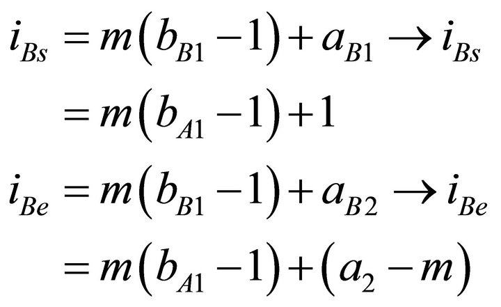
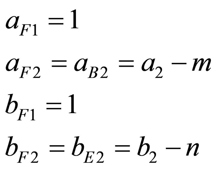
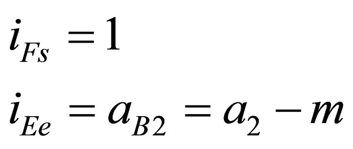
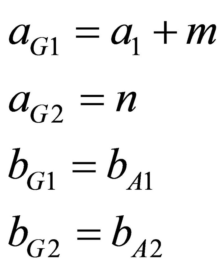
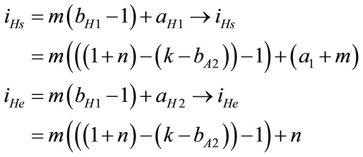
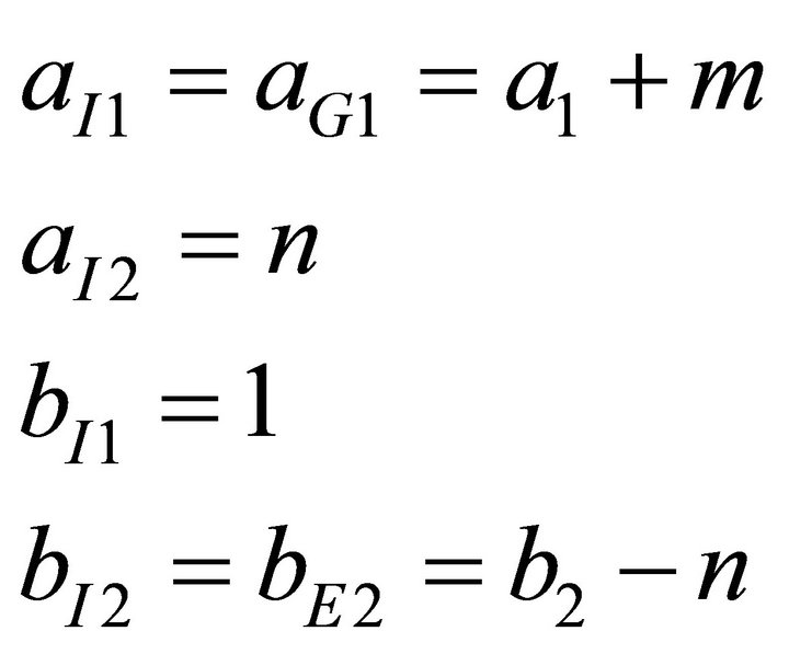
Each section (area) has its own equation-system and its own parameters a, b and i in the equations). Equations and parameters can be traced back to the parameters and equations of section “A”, as it is presented later (equations following the arrows).
After solving equations in Parts 3.3.1 to 3.3.10, the next step is to compute the result of equation in part 3.3.11. It is the average wanted, and it gives the result of the convolution.
Equation-system has to be iterated as the matrix passes on the sub-resolution.
In the following, to understand what equations makes, it is useful to studying Figure 4-6.
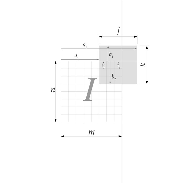
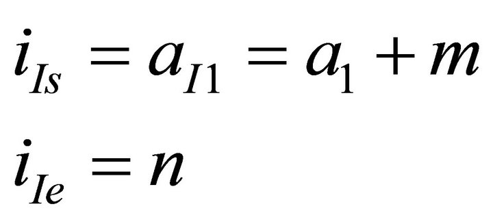
Figure 5. Parameters used when convolving a raster image with sub-resolution. m and n—Number of the columns and rows of the cell I, where I is a cell with sub-resolution of a raster image (see Figure 6). j and k—Number of columns (j) and rows (k) of the convolution matrix (convolving core). a1 and a2—Number of units from the left side of the subresolution to the left side (a1) and the right side (a1) of the convolution matrix. 1 unit = 1 column of the sub-resolution. b1 and b2—Number of units from the top edge of the subresolution to the top edge (b1) and the bottom edge (b2) of the convolution matrix. 1 unit = 1 row of sub-resolution. is and ie—The ordinal number of the column of the subresolution which currently contains the first column (is) and the last column (ie) of the convolution matrix. When first column of convolution matrix is expanded over the current sub-resolution, where value of is has to be equal to 1. When last column of convolution matrix is expanded over the current sub-resolution area, value of ie has to be equal to m.

Figure 6. Adjacent rasters of a cell with sub-resolution: cell I has a sub-resolution, M is the same as on Figure 3. I is an ordinal number of column which currently contains I.
3.3.1. Common Rules
 (6)
(6)
3.3.2. Segment “A” (I)
 (7)
(7)
 (8)
(8)
 (9)
(9)
3.3.3. Segment “B” (I + 1)
 (10)
(10)
 (11)
(11)
 (12)
(12)

 (13)
(13)
3.3.4. Segment “C” (I − M)
 (14)
(14)
 (15)
(15)
 (16)
(16)

 (17)
(17)
3.3.5. Segment “D” (I + 1 − M)
 (18)
(18)
 (19)
(19)
 (20)
(20)

 (21)
(21)
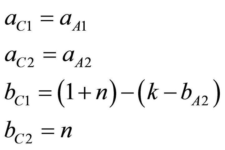
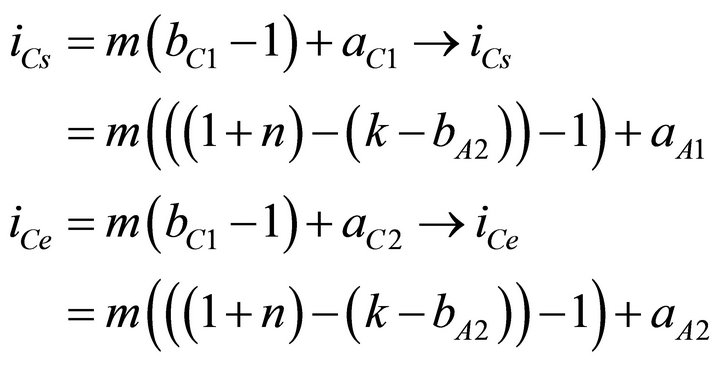
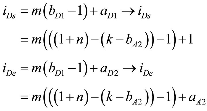
3.3.6. Segment “E” (I + M)
 (23)
(23)
 (24)
(24)

 (25)
(25)

 (26)
(26)
3.3.7. Segment “F” (I + 1 + M)
 (27)
(27)
 (28)
(28)

 (29)
(29)

 (30)
(30)
3.3.8. Segment “G” (I − 1)
 (31)
(31)
 (32)
(32)
 (33)
(33)

 (34)
(34)
3.3.9. Segment “H” (I − 1 − M)
 (35)
(35)
 (36)
(36)
 (37)
(37)

 (38)
(38)
3.3.10. Segment “I” (I − 1 + M)
 (39)
(39)
 (40)
(40)
 (41)
(41)

 (42)
(42)
3.3.11. Average for i
 (43)
(43)
4. Converting an Mrifile into Vector Format
Mri format allows raster-vector conversion, because contains enough data to determinate the center point of each raster cell of each sub-resolution. Current value of parameters XLLCorner, YLLCorner, Height, Width, MyBaseRaster, Columns, Rows, FromX, FromY, NO_DATA, are always known, and they makes possible to compute the center point of every raster cell (Figure 7). The simplest way is probably to create an ASCII point vector file. Resultant vector based model can be used as usual, creating—for example—a TIN-model for 3D visualization.

Figure 7. Example of a point vector map derived from a multiresolution raster image. Origin of this vector map is the raster image b on Figure 2.
5. Further Ways of Development
Multi color resolution in the same image: each subresolution should have its own color model. Practically it only would be a tag in the xml file that contains the color model used. It allows using raster images with different color-model in the same image, so there is no need to convert separate images to the same color-model before importing it. For example:
In this case it is possible to use several color model in the same image, but only one can be used by sub-resolutions. Let might prove to be an important question, how to perform computations when two or more different model have to be considered at the same time?
Extended multiresolution: each sub-resolution should have different resolutions. This would give the maximum flexibility in the practice; on the other hand there would be many problems in the field of image analysis and image processing. The storage of attribute data would be very simple in the file structure presented in this paper, because xml tag allow to define different resolutions by the using sub-resoultions.
The question naturally arises, how to make computations (for example: convolution) when rasters with different sub-resolutions are adjacent? What to do when its quotation is not an integer?
3D mri. This would be very useful in 3D GIS, for example in the field of geological modeling, or meteorological modeling. The basis idea is the same as in the 2D mri, and the file structure would be similar. The main problem is the mathematical background, equations and thoughts presented in this paper probably would be inadequate in this case.
6. Summary
In the field of surveying and GIS based spatial analysis it is a common problem to use a raster images simultaneously with two or more different resolution. This problem can be divided in two parts: storing of the image and perform mathematical operations on it.
Our research gives a possible solution for this situation, because multiresolution image format (mri) allows
• to store raster based images with different resolution in the same file and in the same time;
• to import or export easily any part of the image as a separate image;
• to define geographical reference for a raster image and use this image as a raster based GIS model;
• to perform computations (i.e., image manipulation) on the content of the file.
Moreover, mri format allows a wide compatibility and interoperatibility, since it is a text file, conformed to xml 1.0 standard.
As we have shown it is possible to perform mathematical operations on an mri file, presented an algorithm and the proper equations to execute a convolution and we alluded to the possibility of conversion a multiresolution raster into vector format.
In the practice, mri format should be very useful, not only in the field of GIS, but also in the field of the general image storing and processing. Mri allows to take multiresolutional photos and videos, or security cameras, when only a moving object has to be stored using the full resolution while the background may be stored with lower resolution.
As for further development of mri format, we suggested three main point:
• multi color resolution• extendend multiresolution• 3D multiresolution.
Naturally, any further ways of development of mri format and ideas would be appreciated by the authors.
7. Acknowledgements
Many thanks to Mr. PERE László programmer, mathematician (Blum Software Engineering Ltd., Hungary), for thought-provoking reviews, constructive comments and the linguistic support.
REFERENCES
- T. K. Peucker, R. J. Fowler, J. J. Little and D. M. Mark, “The Triangulated Irregular Network,” Proceedings of the ASP-ACSM Symposium on DTM's, St. Louis, 1978, pp. 516-540.
- T. Bray, J. Paoli, C. M. Sperberg-McQueen, E. Maler and Y. François, “Extensible Markup Language (XML) 1.0 (Fifth Edition),” 2008. http://www.w3.org/TR/2008/REC-xml-20081126/
- B. Antoniou and L. Tsoulos, “The Potential of XML Encoding in Geomatics Converting Raster Images to XML and SVG,” Computers & Geosciences, Vol. 32, No. 2, 2006, pp. 184-194. doi:10.1016/j.cageo.2005.06.004
NOTES
1Our proposal is to using mri as file extension for multiresolution images. Mri (magnetic resonance imaging) as method used by medical imaging uses dicom format and uses not mri as extension.
2By default Height and Width has the same value.