Natural Science
Vol.4 No.8(2012), Article ID:22001,7 pages DOI:10.4236/ns.2012.48077
Solving high-order nonlinear Volterra-Fredholm integro-differential equations by differential transform method
![]()
General Required Courses Department, Jeddah Community College, King Abdulaziz University, Jeddah, KSA; salah_behiry@hotmail.com, drsaied1957@gmail.com
Received 30 May 2012; revised 28 June 2012; accepted 12 July 2012
Keywords: Differential transform method; Volterra-Fredholm integro-differential equations
ABSTRACT
In this paper, we apply the differential transformation method to high-order nonlinear VolterraFredholm integro-differential equations with separable kernels. Some different examples are considered the results of these examples indicated that the procedure of the differential transformation method is simple and effective, and could provide an accurate approximate solution or exact solution.
1. INTRODUCTION
Integral and integro-differential equations play an important role in characterizing many social, biological, physical and engineering problems; for more details see [1-3] and references cited therein. Nonlinear integral and integro-differential equations are usually hard to solve analytically and exact solutions are rather difficult to be obtained. Many numerical methods have been studied such as the Legendre wavelets method [4], the Haar functions method [5,6], the linearization method [7], the finite difference method [8], the Tau method [9,10], the hybrid Legendre polynomials and block-pulse functions [11], the Adomian decomposition method [12,13], the Taylor polynomial method [14-16] and the collocation approach (for linear case) [17].
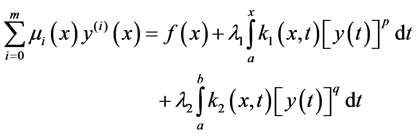
In this paper, we will use the differential transform method (DTM) to solve a high-order nonlinear VolterraFredholm integro-differential equation given by
 ,(1.1)
with the initial conditions
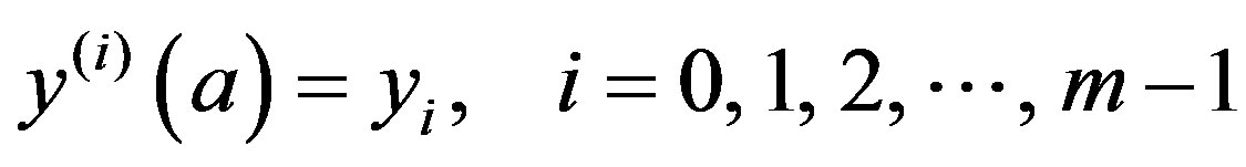 ,(1.2)
where  are constant values,
  ,
,  ,
,  and
and  with
with  are known functions that have suitable derivatives on an interval
 ,
,  are integers and
  is the unknown function. The concept of the DTM was first proposed by Zhou [18] and has been used to solve both linear and nonlinear initial value problems, in electric circuit analysis. The DTM is a distinguished form of the Taylor series method, which requires symbolic computation of the necessary derivatives of the data functions. Taylor polynomials method is computationally tedious for high orders. DTM leads to an iterative procedure for obtaining an analytic series solution of functional equations. It is possible to solve differential equations, difference equations, differential difference equations, fractional differential equations, pantograph equations, integral equations and integro-differential equations by using this method.
In this work, we apply the DTM to solve high-order nonlinear Volterra-Fredholm integro-differential equations with separable (degenerate) kernels; i.e.  . Five different problems are solved to make clear the application of the DTM on such class of integro-differential equations. We introduce theorems in general forms to be able to apply any kind of integro-differential in any order.
2. DIFFERENTIAL TRANSFORM METHOD
The basic definition and the fundamental theorems of the differential transformation and its applicability for various kinds of differential and integral equations are given in [19-22]. For convenience of the reader, a review of differential transformation will be presented here. The transformation of the kth derivative of a function in one variable is as follows.
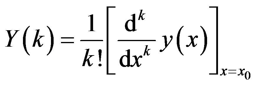 , (2.1)
and the inverse transformation is defined by
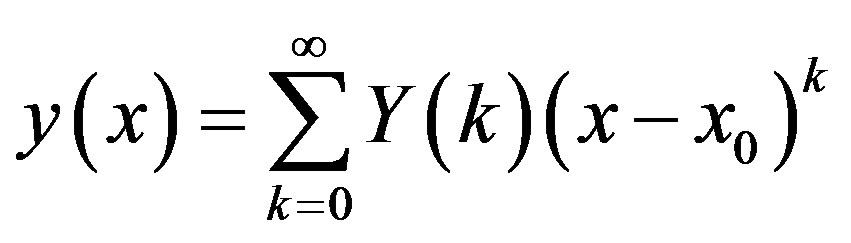 . (2.2)
The following theorems can be deduced from eqs.2.1 and 2.2.
Theorem 1. If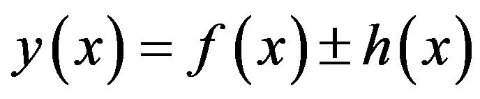 , then
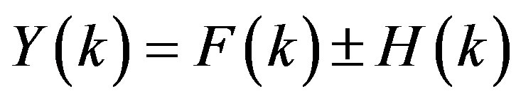 .
.
Theorem 2. If , then
 , where
  is a constant.
Theorem 3. If , then
 .
.
Theorem 4. If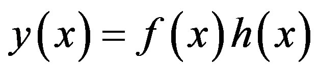 , then
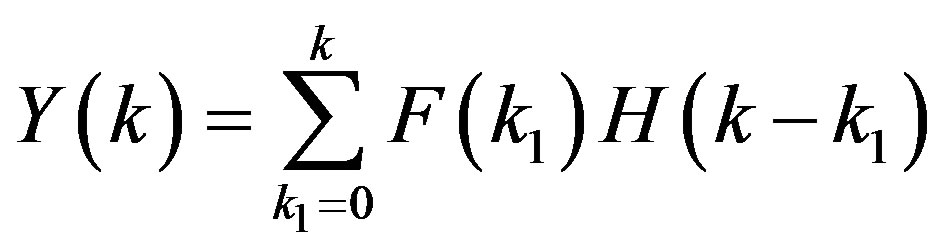 .
.
Theorem 5. If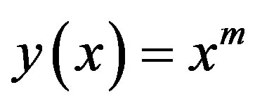 , then
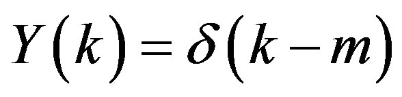 , where
 .
.
Theorem 6. If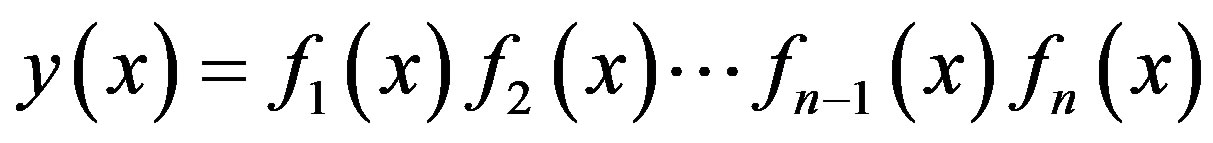 , then
 .
.
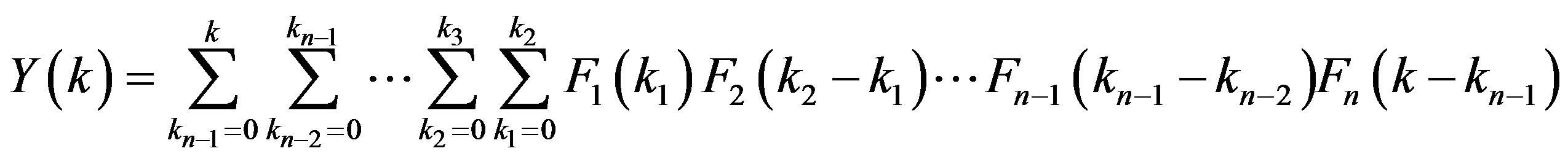
Theorem 7. If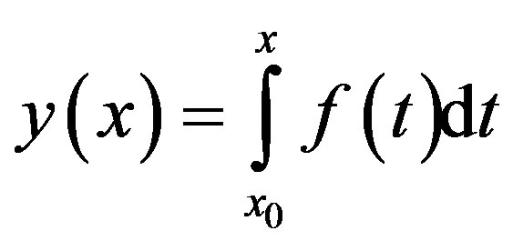 , then
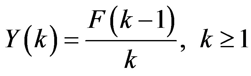 .
.
Theorem 8. If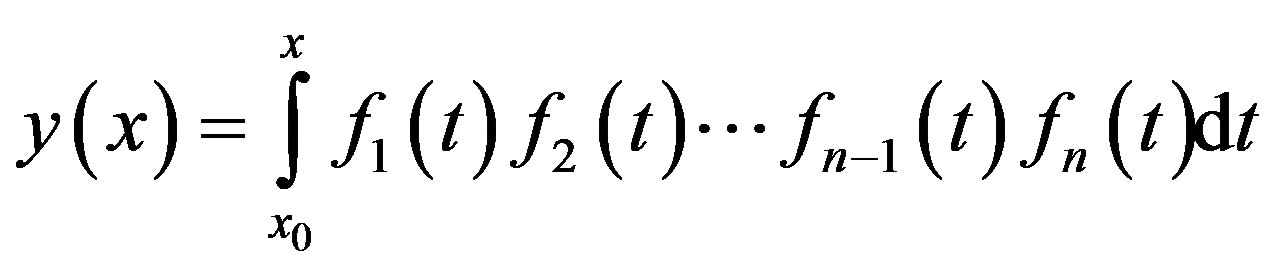 , then

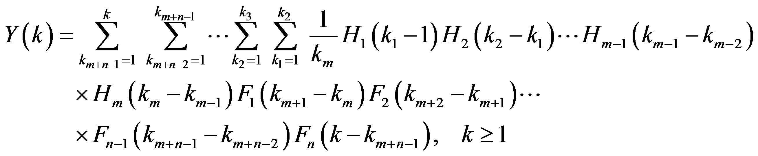
Theorem 9. If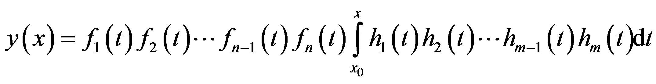 , then
The following relation is quite useful in the solution of Fredholm integrals; it can be obtained from theorem 8 and eq.2.2
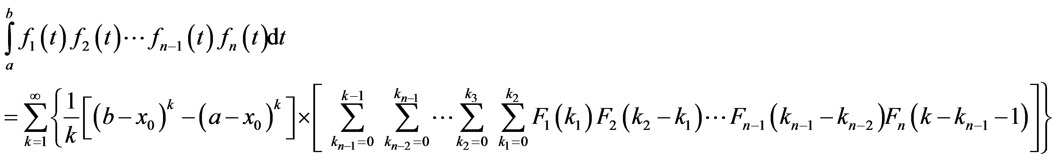 (2.3)
(2.3)
Also, we introduce the differential transformations for some basic functions, which are encountered in the following examples. The proof of these differential transforms follows directly from the definition (2.1) and (2.2) and the operations of the differential transformation given in the above theorems.
• If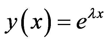 , then
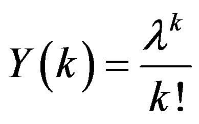 .
.
• If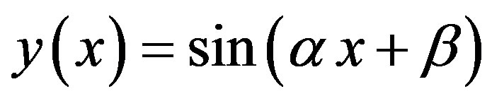 , then
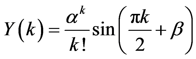 .
.
• If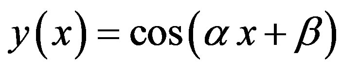 , then
 .
.
3. APPLICATIONS AND NUMERICAL RESULTS
In this section, we implement the DTM on some different examples.
Example 3.1. Consider the nonlinear Volterra-Fredholm integro-differential equation
 (3.1)
(3.1)
with the initial conditions
 (3.2)
(3.2)
Application of the differential transform to eq.3.1 gives
 (3.3)
(3.3)
where .
.
Substitute  and 6 into eq.3.3, one can get the following relations
 ,
,
 ,
,
 ,
,
 ,
,
 and
and
Also, for  in eq.3.3, the following recurrence relation can be obtained
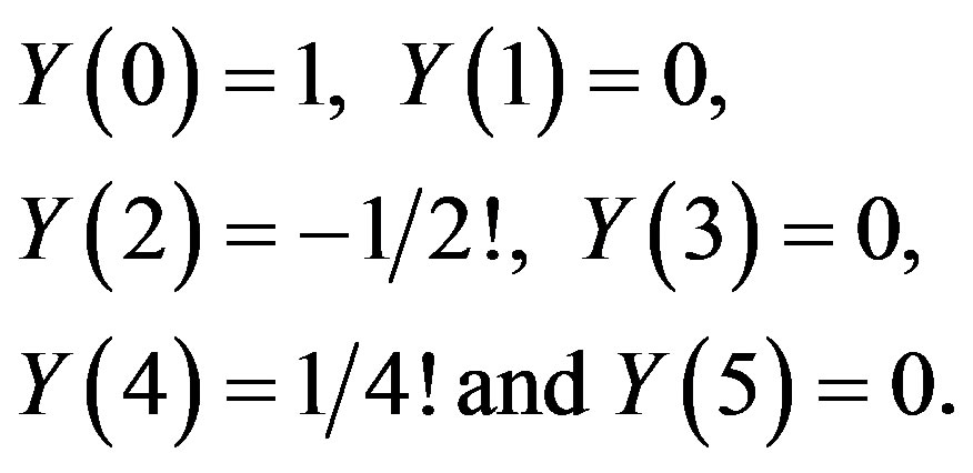
The initial conditions in eq.3.2 is transformed by using (2.1) to

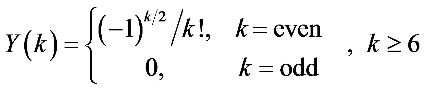
Consequently, from the above recurrence relations we can easily find that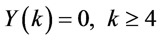 .
.
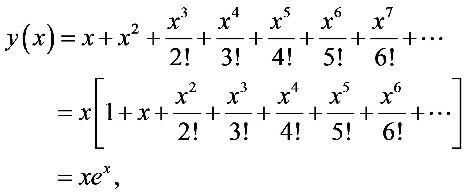
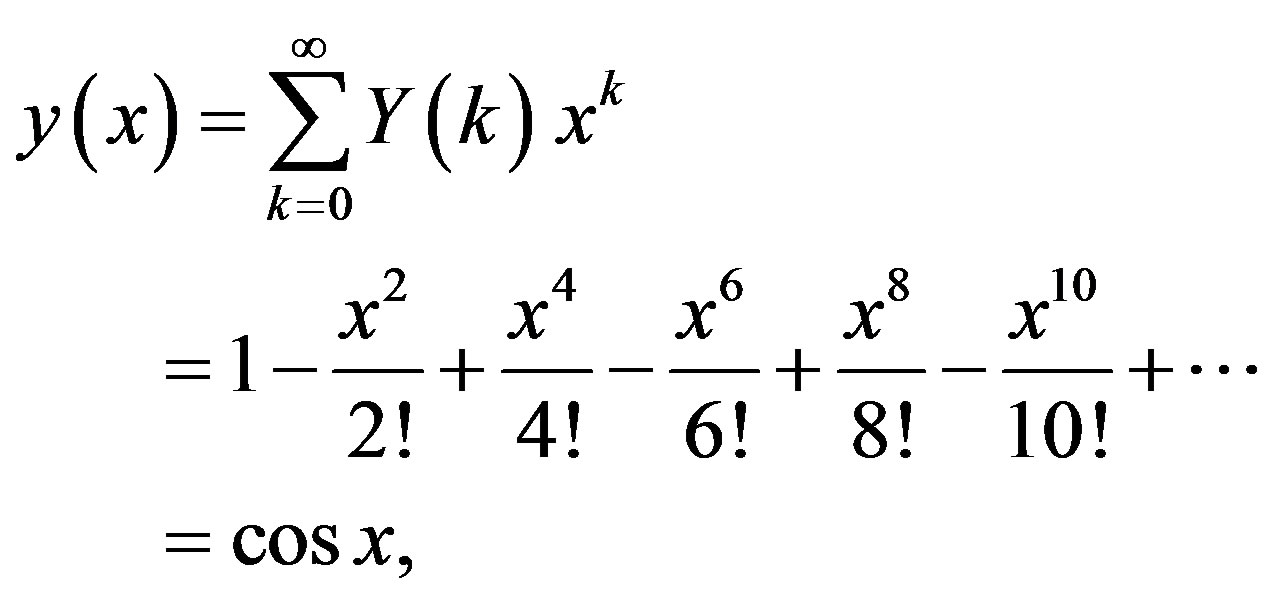
Hence by using eq.2.2, the solution of the integrodifferential eq.3.1 with its initial conditions (3.2) is obtained to be
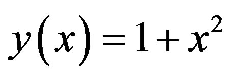 which is the exact solution.
Example 3.2. Consider the integro-differential equation
 (3.4)
(3.4)
with the initial conditions
 (3.5)
(3.5)
The differential transformation of eq.3.4 and the initial conditions (3.5) are
 (3.6)
(3.6)
where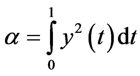 , and
, and
 (3.7)
(3.7)
Utilizing the recurrence relation (3.6) and the transformed initial conditions (3.7), we can obtain
Substitute  into eq.2.2 to obtain the solution of the nonlinear Volterra-Fredholm integro-differential equation in this example
which is its exact solution.
Example 3.3. Consider the following sixth order Volterra-Fredholm integro-differential equation
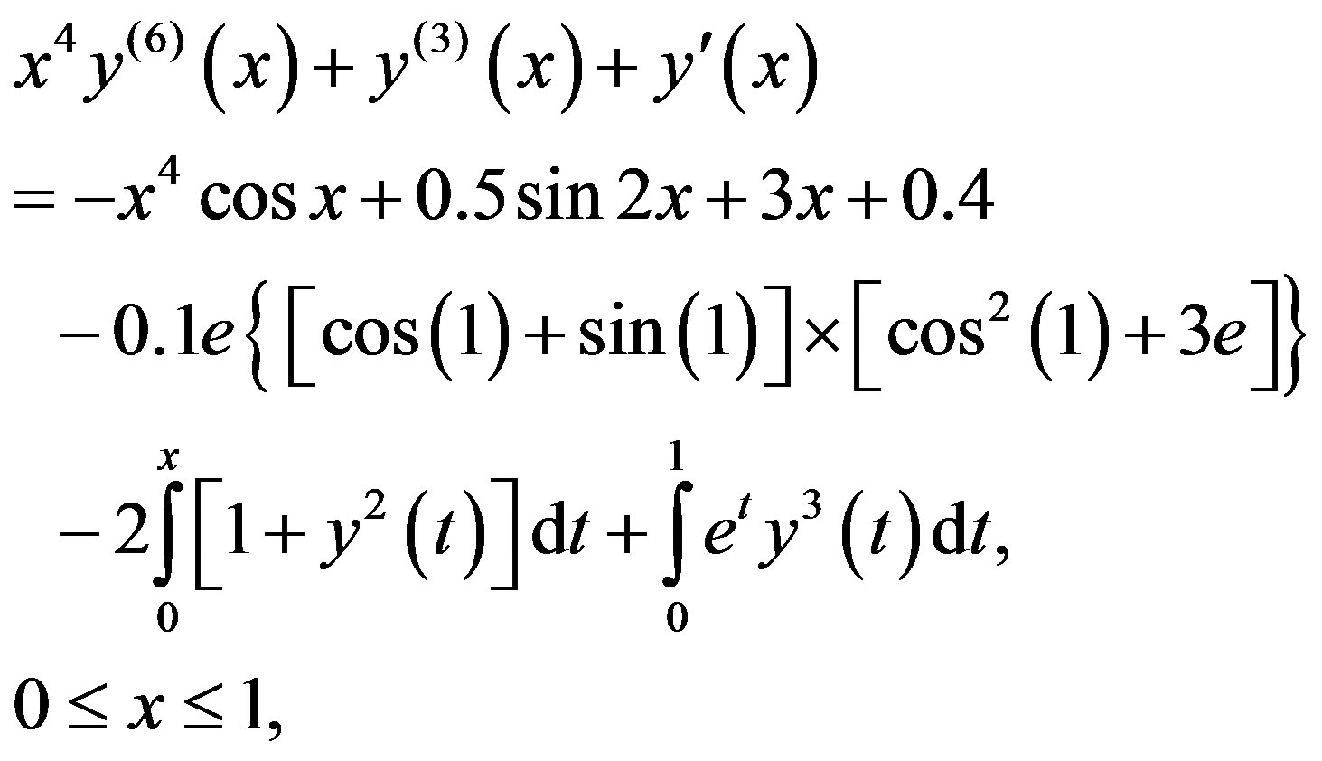 (3.8)
(3.8)
with the initial conditions
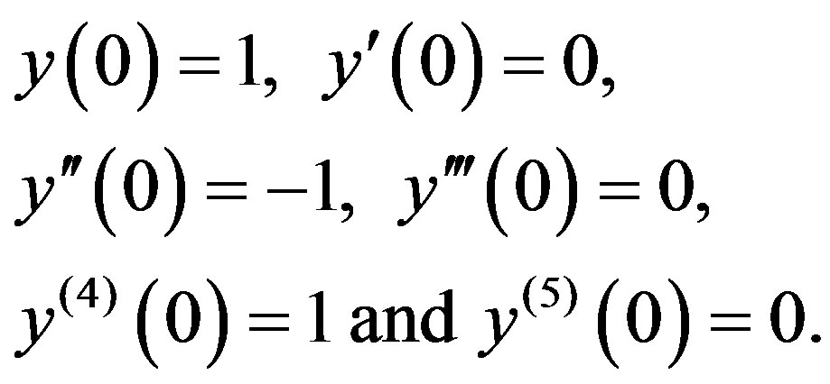 (3.9)
(3.9)
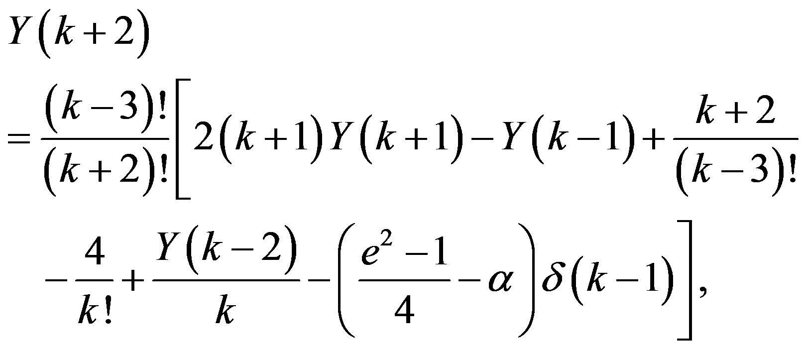
The differential transformation of eq.3.8 and the initial conditions (3.9) are
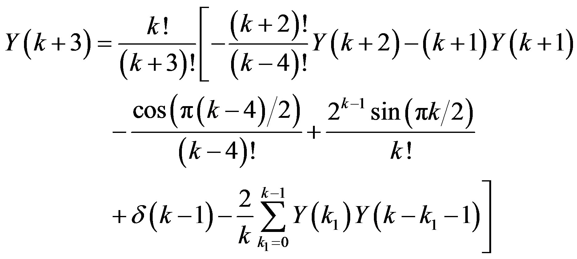 (3.10)
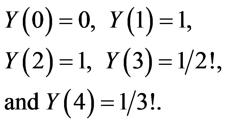
and
 (3.11)
Note that, in eq.3.10 the first and third terms in left hand side vanish as .
.
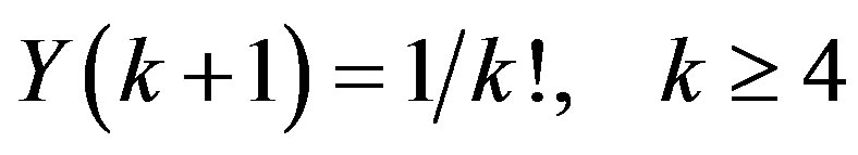
Utilizing the recurrence relation (3.10) and the transformed initial conditions (3.11), we can get
Therefore, the solution of eq.3.8 is given by
which is the exact solution.
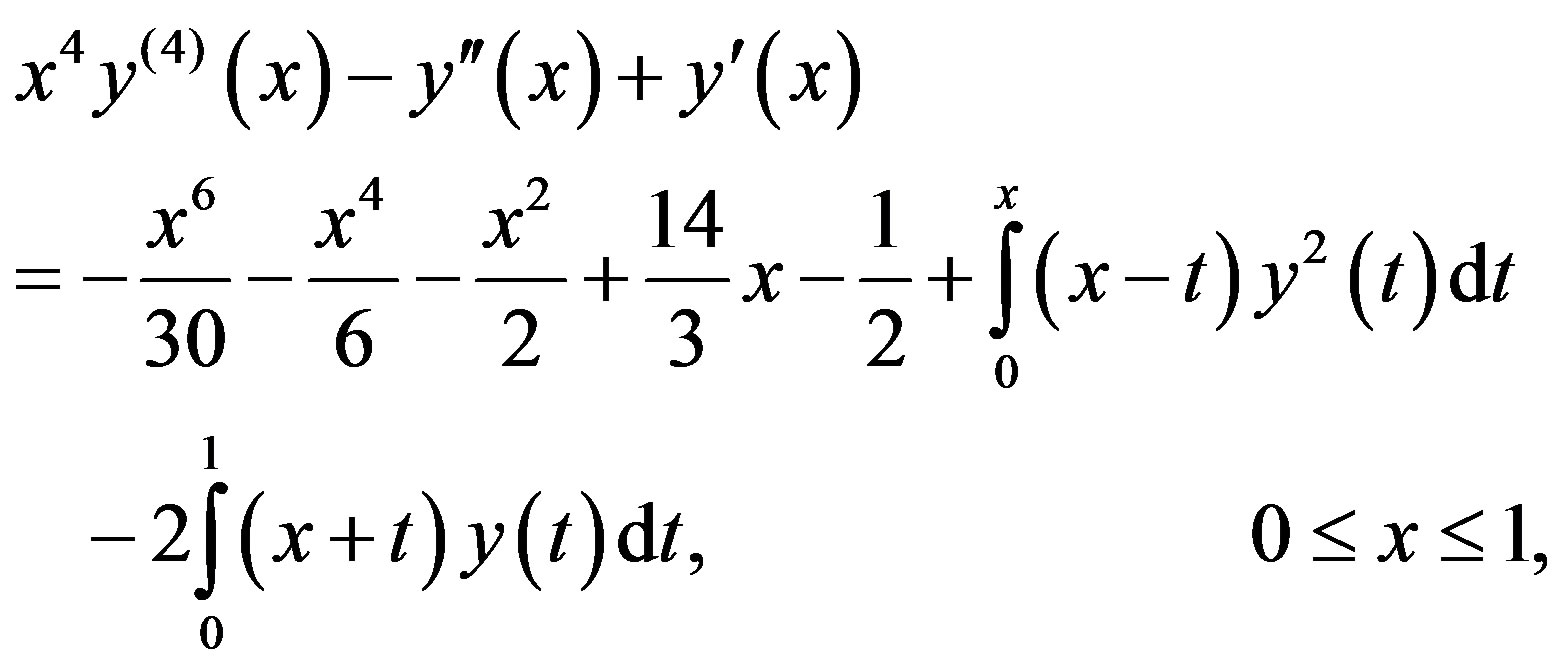
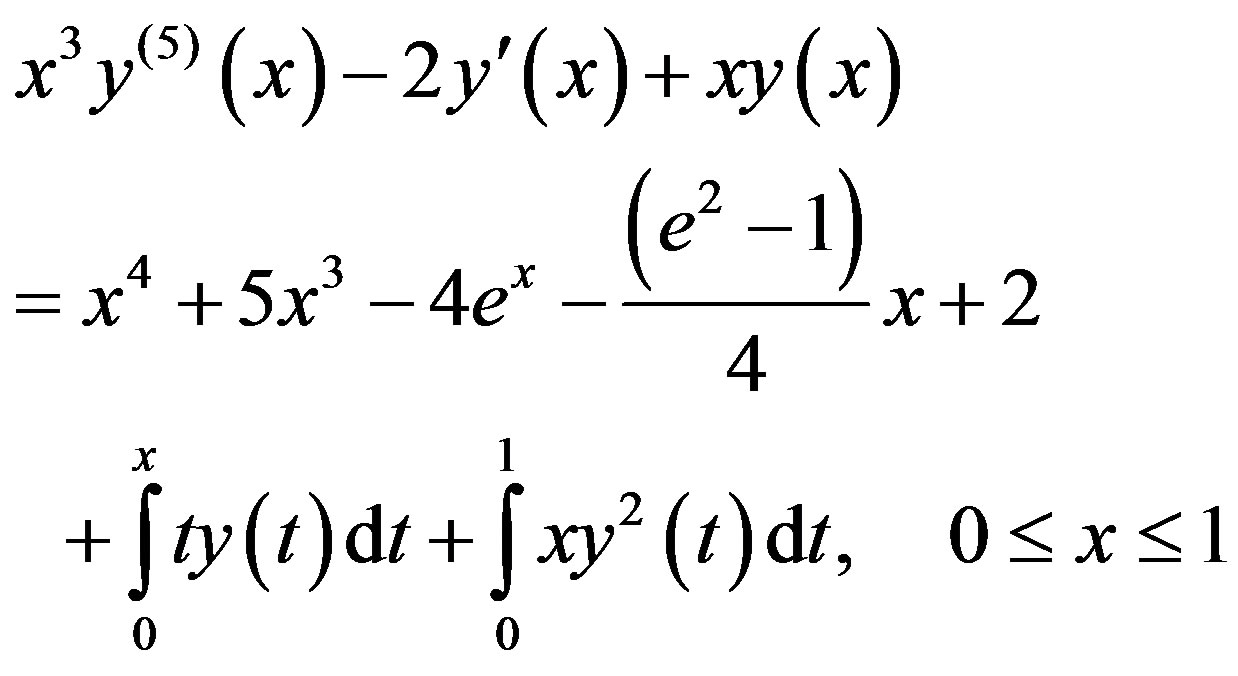
Example 3.4. Let us consider the nonlinear VolterraFredholm integro-differential equation [23]
 (3.12)
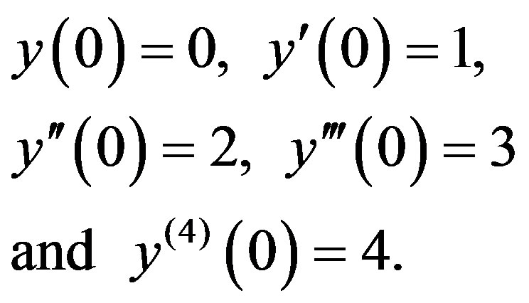
with the initial conditions
 (3.13)
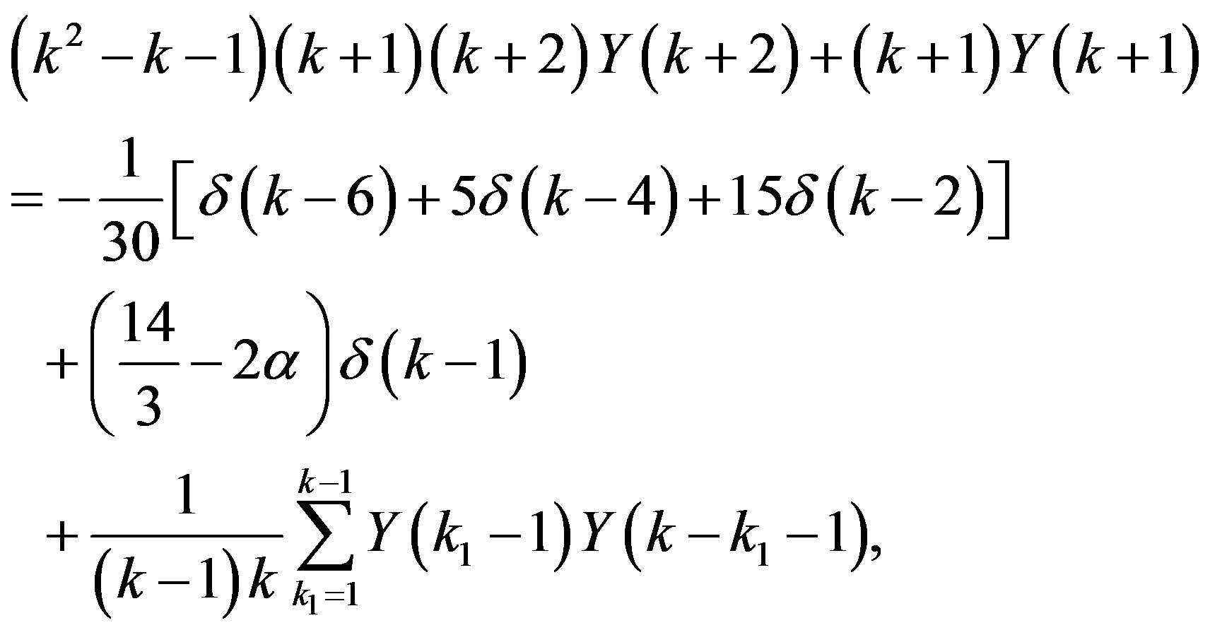
The differential transformation of this equation and its initial conditions are
 (3.14)
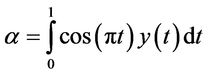
where
 , (3.15)
 (3.16)
and
 (3.17)
To obtain , put
, put  into eq.3.12 and utilizing the transformation (2.1), hence
 .
.
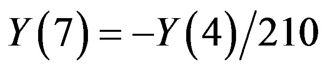
Substitute  and 5 into eq.3.14, one can get the following relations
 , (3.18)
 , (3.19)
 ,
,  , and
, and 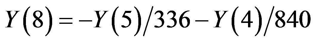 .
.
Also, for  in eq.3.14, the following recurrence relation can be obtained
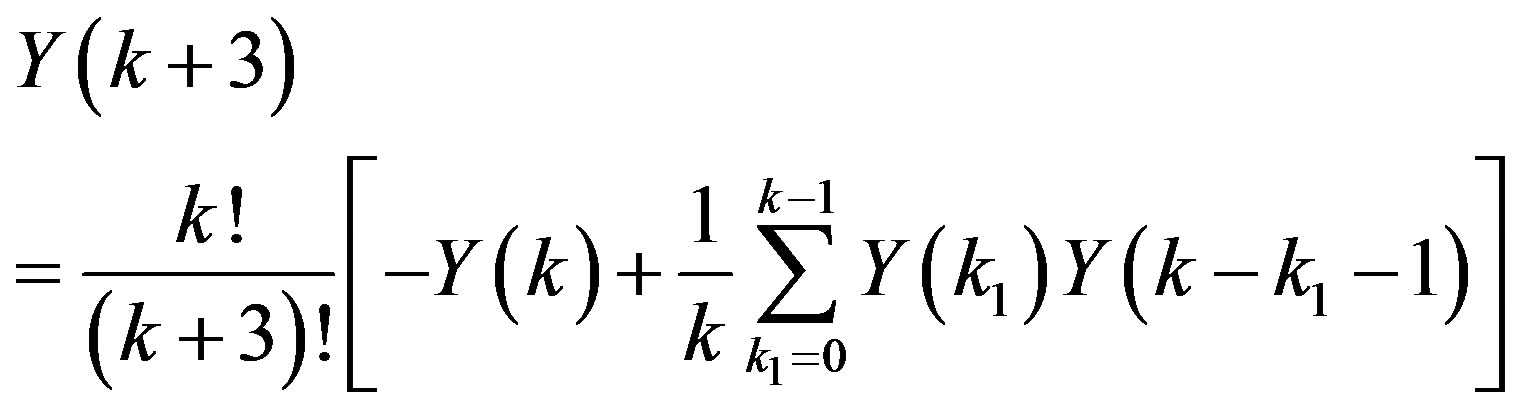 .
.
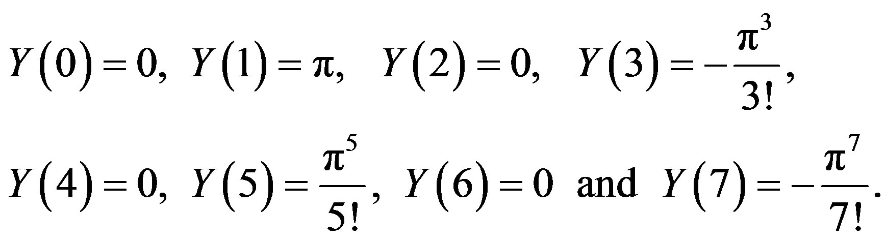
Utilizing eqs.2.3, 3.15 and 3.16, it can be shown that the following equalities hold for  and
and 
 , (3.20)
 , (3.21)
where  is a suitably large integer that represents the number of terms to be chosen. Solving eqs.3.20 and 3.21 with eqs.3.18 and 3.19 by taking
  terms, one can obtain the following results
 ,
,  ,
,  and
and .
.
Hence one can get all the missing coefficients of  of the expansion for the unknown function, that is
 which is the exact solution.
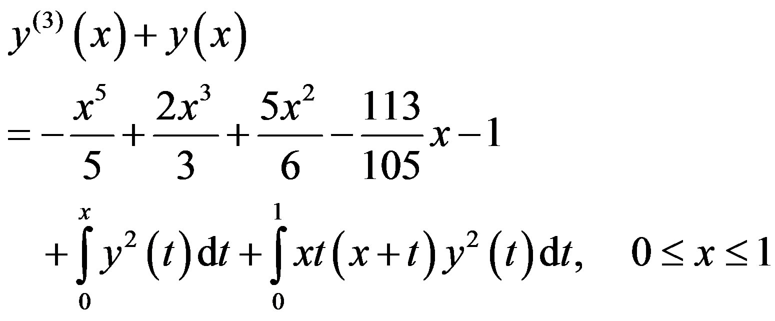
Example 3.5. Consider the nonlinear Volterra-Fredholm integro-differential equation
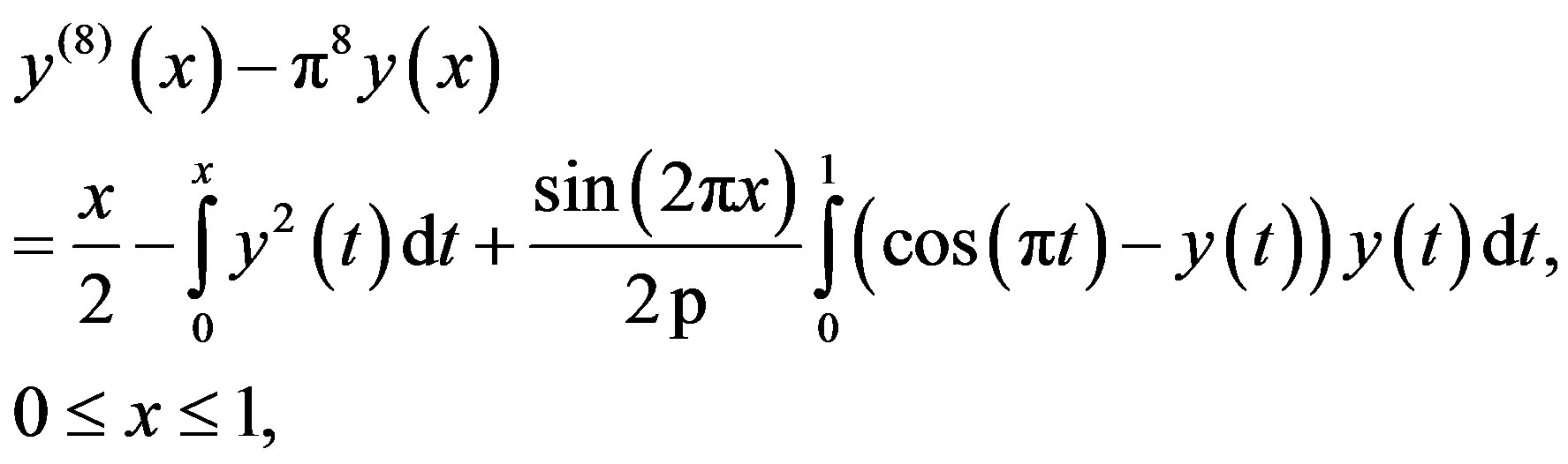 (3.22)
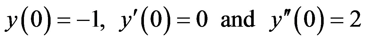
with the initial conditions
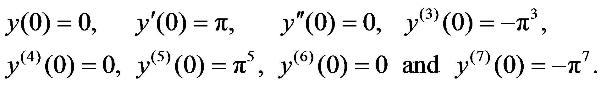 (3.23)
Eq.3.22 can be written in the following form
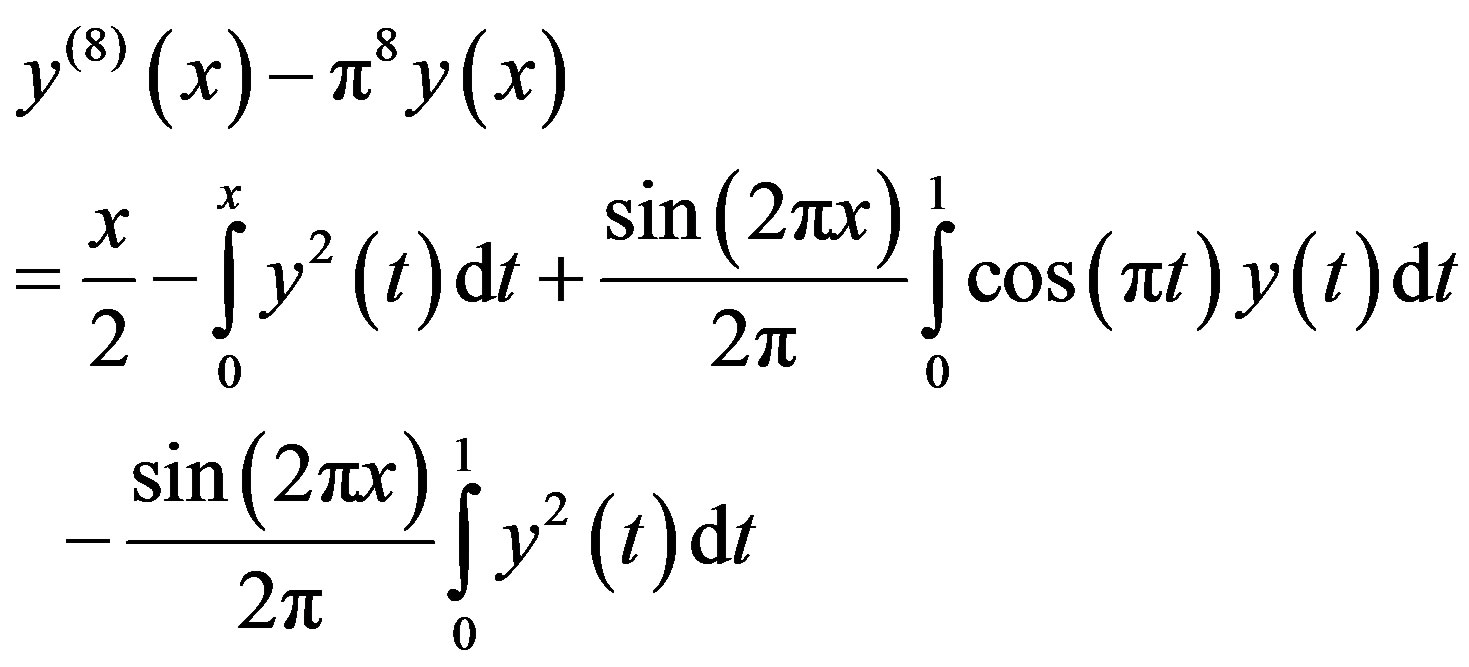 (3.24)
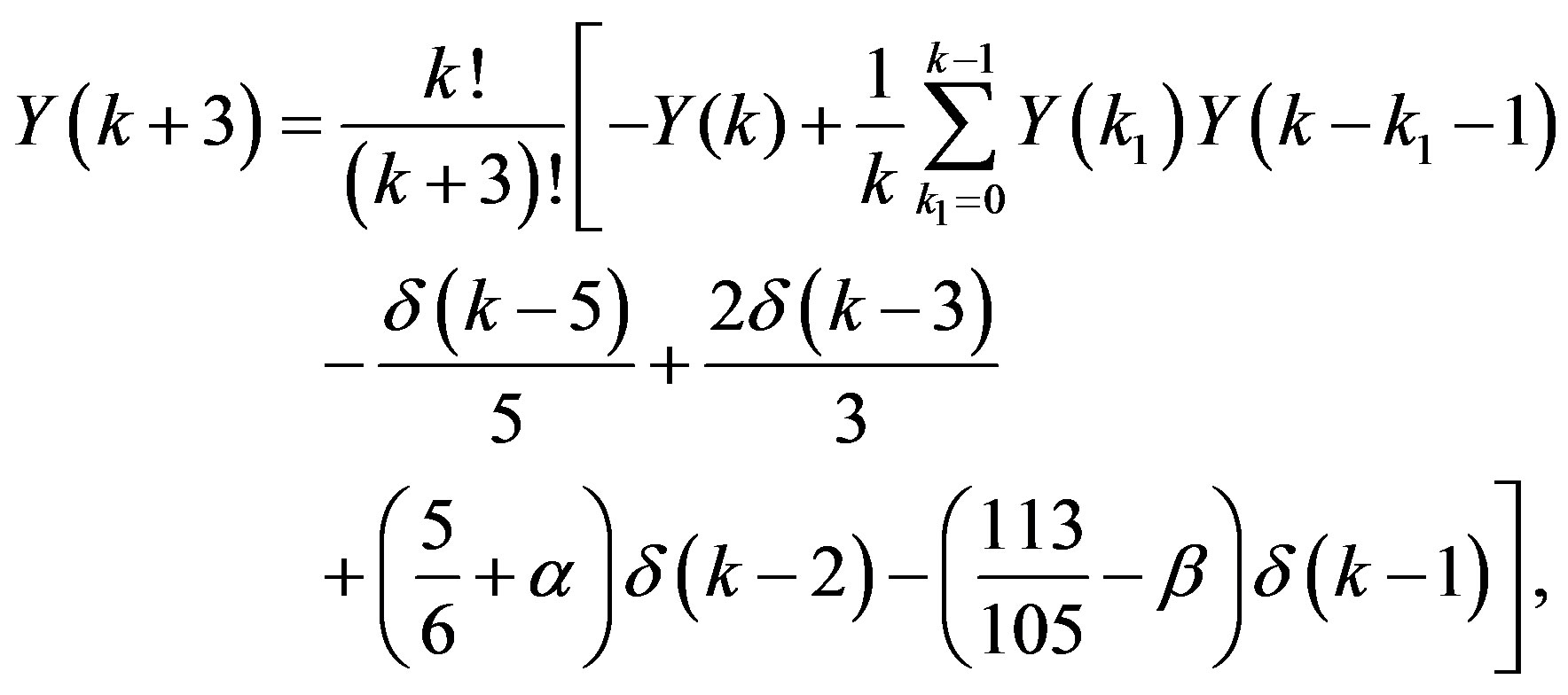
The differential transformation of the eq.3.24 gives the following recurrence relation
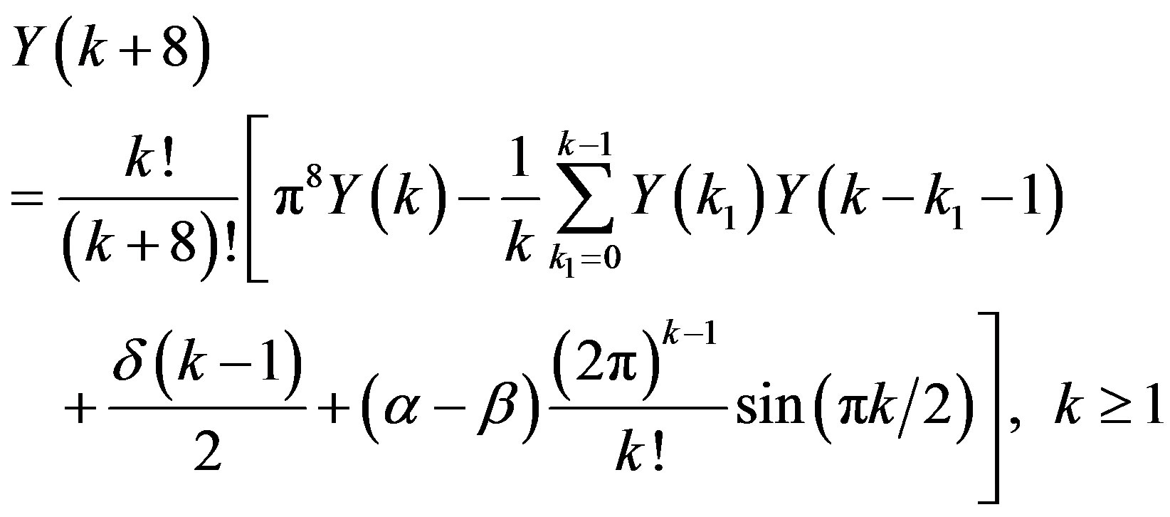 (3.25)
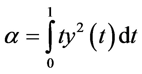
where
 , and
, and 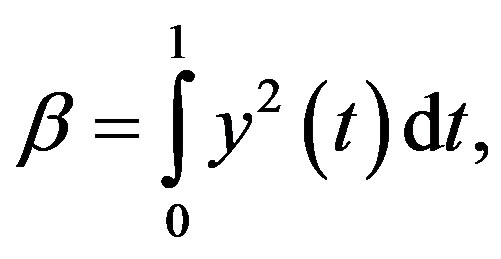 (3.26)
The initial conditions in eq.3.23 are transformed by using eq.2.1 as follows
 (3.27)
Also, for obtaining , put
, put  into eq.3.22 and utilize (2.1), one can get
 . (3.28)
By using the transformed initial conditions in (3.27) and (3.28) and the recurrence relation in eq.3.25, the series solution is then evaluated for  up to
up to 
 (3.29)
Utilizing eqs.2.3 and 3.26, one can show
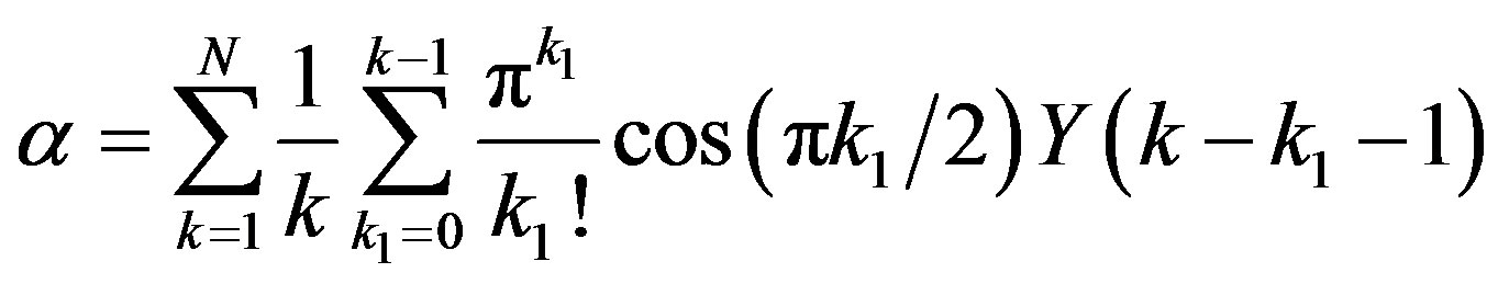 , (3.30)
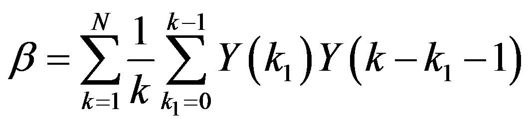 , (3.31)
where  is a sufficiently large integer. Solving eqs. 3.30 and 3.31 by taking
  terms, we can get
 , and
, and .
.
The unknown function is evaluated by using eq.3.29 for these values of  and
and . The numerical results are shown in Table 1 with comparison to the exact solution
 .
.
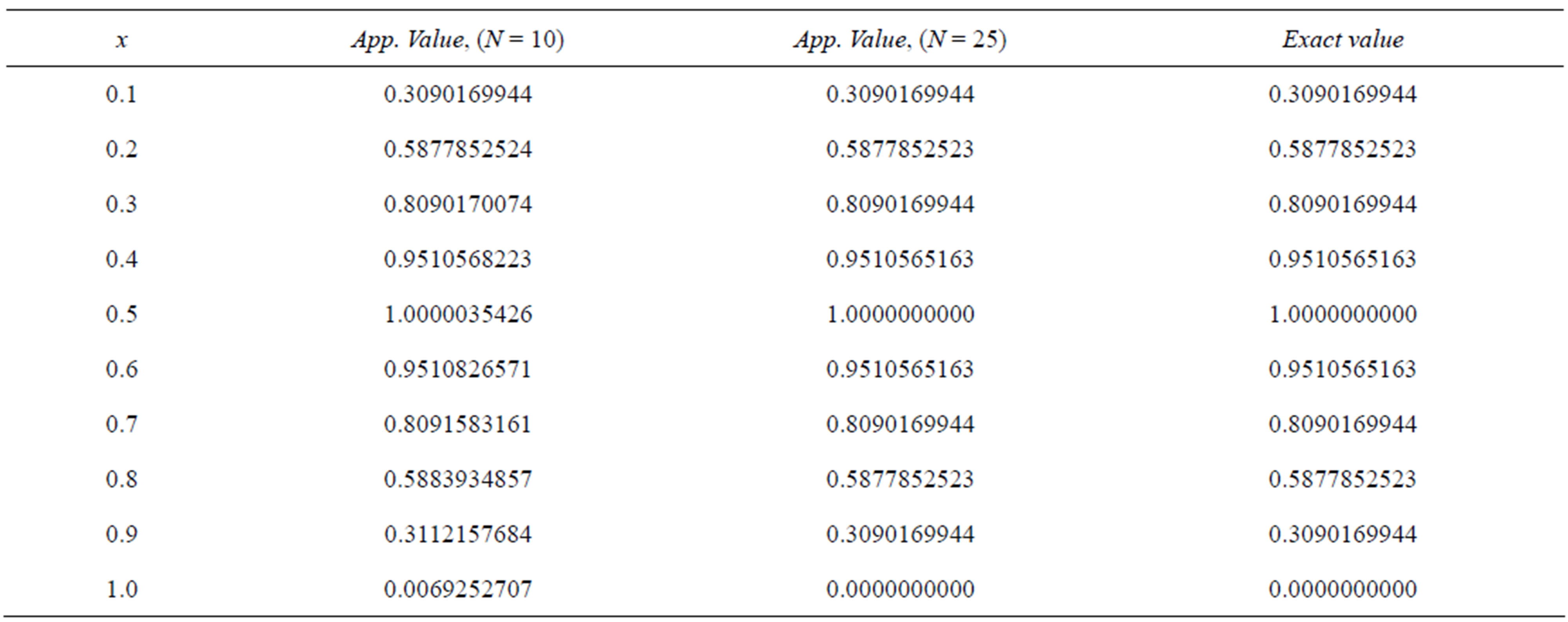
Table 1. Numerical comparison of results in example 3.5.
4. CONCLUSION
In this work, the differential transform method for the solution of high-order nonlinear Volterra-Fredholm integro-differential equations is successfully implemented. The present method reduces the computational difficulties of other traditional methods and all the calculation can be made simple manipulations. The accuracy of the obtained solution can be improved by taking more terms in the solution. In many cases, the series solution obtained with differential transform method can be written in exact closed form.
REFERENCES
- Kythe, P.K. and Puri, P. (1992) Computational methods for linear integral equations. University of New Orleans, New Orleans.
- Wazwaz, A.M. (2006) A comparison study between the modified decomposition method and traditional method. Applied Mathematics and Computation, 181, 1703-1712. doi:10.1016/j.amc.2006.03.023
- Rashed, M.T. (2004) Numerical solution of functional differential, integral and integro-differential equations. Applied Numerical Mathematics, 156, 485-492.
- Razzaghi, M. and Yousefi, S. (2005) Legendre wavelets method for nonlinear Volterra-Fredholm integral equations. Mathematics and Computers in Simulation, 70, 1-8. doi:10.1016/j.matcom.2005.02.035
- Maleknejed, K. and Mirzaee, F. (2006) Numerical solution of integro-differential equations by using rationalized Haar functions method. Kybernetes, 35, 1735-1744. doi:10.1108/03684920610688694
- Reihani, M.H. and Abadi, Z. (2007) Rationalized Haar functions method for solving Fredholm and Volterra integral equations. Journal of Computational and Applied Mathematics, 200, 12-20. doi:10.1016/j.cam.2005.12.026
- Darania, P., Abadian, E. and Oskoi, A.V. (2006) Linearization method for solving nonlinear integral equations. Mathematical Problems in Engineering, 1-10. doi:10.1155/MPE/2006/73714
- Zhao, J. and Corless, R.M. (2006) Compact finite difference method for integro-differential equations. Applied Mathematics and Computation, 177, 271-288. doi:10.1016/j.amc.2005.11.007
- Abbasbandy, S. and Taati, A. (2009) Numerical solution of the system of nonlinear Volterra integro-differential equations with nonlinear differential part by the operational Tau method and error estimation. Journal of Computational and Applied Mathematics, 231, 106-113. doi:10.1016/j.cam.2009.02.014
- Ebadi, G., Rahimi-Ardabili, M. Y. and Shahmorad, S. (2007) Numerical solution of the nonlinear Volterra integro-differential equations by the Tau method. Applied Mathematics and Computation, 188, 1580-1586. doi:10.1016/j.amc.2006.11.024
- Maleknejad, K., Basirat, B. and Hashemizadeh, E. (2011) Hybrid Legendre polynomials and Block-pulse functions approach for nonlinear Volterra-Fredholm integro-differential equations. Computers & Mathematics with Applications, 61, 2821-2828. doi:10.1016/j.camwa.2011.03.055
- Wazwaz, A.M. (2010) The combined Laplace transformAdomian decomposition method for handling nonlinear Volterra integro-differential equations. Applied Mathematics and Computation, 216, 1304-1309. doi:10.1016/j.amc.2010.02.023
- Araghi, M.A. and Behzadi, Sh.S. (2009) Solving nonlinear Volterra-Fredholm integro-differential equations using the modified Adomian decomposition method. Computational Methods in Applied Mathematics, 9, 321-331.
- Darania, P. and Ivaz, K. (2008) Numerical solution of nonlinear Volterra-Fredholm integro-differential equations. Applied Mathematics and Computation, 56, 2197- 2209. doi:10.1016/j.camwa.2008.03.045
- Maleknejad, K. and Mohmoudi, Y. (2003) Taylor polynomial solution of high-order nonlinear Volterra-Fredholm integro-differential equations. Applied Mathematics and Computation, 145, 641-653. doi:10.1016/S0096-3003(03)00152-8
- Yalcinbas, S. (2002) Taylor polynomial solution of nonlinear Volterra-Fredholm integral equations. Applied Mathematics and Computation, 127, 195-206. doi:10.1016/S0096-3003(00)00165-X
- Yüzbaşi, Ş., Şahin, N. and Yildirim, A. (2012) A collocation approach for solving high-order linear FredholmVolterra integro-differential equations. Mathematical and Computer Modelling, 55, 547-563. doi:10.1016/j.mcm.2011.08.032
- Zhou, J.K. (1986) Differential transformation and its applications for electrical circuits. Huazhong University Press, Wuhan.
- Arikoglu, A. and Ozkol, I. (2005) Solution of boundary value problems for integro-differential equations by using differential transform method. Applied Mathematics and Computation, 168, 1145-1158. doi:10.1016/j.amc.2004.10.009
- Arikoglu, A. and Ozkol, I. (2008) Solution of integral and integro-differential equation systems by using differential transform method. Computers & Mathematics with Applications, 65, 2411-2417. doi:10.1016/j.camwa.2008.05.017
- Odibat, Z.M. (2008) Differential transform method for solving Volterra integral equation with separable kernels. Mathematical and Computer Modelling, 48, 1144-1149. doi:10.1016/j.mcm.2007.12.022
- Biazar, J. and Eslami, M. (2011) Differential transform method for systems of Volterra integral equations of the second kind and comparison with homotopy perturbation method. International Journal of Physical Sciences, 6, 1207-1212.
- Wang, W. (2006) An algorithm for solving the high-order nonlinear Volterra-Fredholm integro-differential equation with mechanization. Applied Mathematics and Computation, 172, 1-23. doi:10.1016/j.amc.2005.01.116