Received 16 September 2014; revised 10 October 2014; accepted 25 October 2014

ABSTRACT

In this paper, we consider cooperative hyperbolic systems involving Schrödinger operator defined on. First we prove the existence and uniqueness of the state for these systems. Then we find the necessary and sufficient conditions of optimal control for such systems of the boundary type. We also find the necessary and sufficient conditions of optimal control for same systems when the observation is on the boundary.

Keywords:

Hyperbolic Systems, Schrödinger Operator, Boundary Control Problem, Boundary Observation, Cooperative

1. Introduction

The optimal control problems of distributed systems involving Schrödinger operator have been widely discussed in many papers. One of the first studies was introduced by Serag [1] , which discusses 2 × 2 cooperative systems of elliptic operator. Further research in this area developed the problem by studying different operator types (el- liptic, parabolic, or hyperbolic) or higher system degree as in [2] - [6] . Many boundary control problems have been introduced in [7] - [10] .

In [3] , we discussed distributed control problem for 2 × 2 cooperative hyperbolic systems involving Schrö- dinger operator.

Here, using the theory of [11] , we consider the following 2 × 2 cooperative hyperbolic systems involving Schrö- dinger operator:

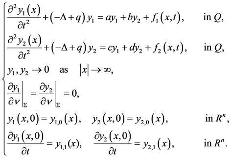(1)

with.

where, , and are given numbers such that, ,

i.e. the system (1) is called cooperative (2)

is a positive function and tending to at infinity, (3)

and with boundary.

The model of the system (1) is given by:

since,.

We first prove the existence and uniqueness of the state for these systems, then we introduce the optimality conditions of boundary control, we also discuss them when the observation is on the boundary.

2. Some Concepts and Results

Here we shall consider some results about the following eigenvalue problem which introduced in [1] and [12] :

(4)

The associated space is, with respect to the norm:

(5)

Since the imbedding of into is compact, then the operator considered as an

Operator in is positive self-adjoint with compact inverse. Hence its spectrum consists of an infinite se- quence of positive eigenvalues, tending to infinity; moreover the smallest one which is called the principal ei- genvalue denoted by is simple and is associated with an eigenfunction which does not change sign in. It is characterized by:

(6)

We have:

which is continuous and compact.

Let us introduce the space of measurable function which is defined on open interval and the variable, denotes the time.

On with Lebesgue measure we have the norm:

and the scalar product

,

the space with the scalar product and the norm above is a Hilbert space.

Analogously, we can define the spaces,

with the scalar product:

then we have:

3. The Existence and Uniqueness for the State of the System (1)

We have the bilinear form:

(7)

For all the function is measurable on.

The coerciveness condition of the bilinear form (7) in has been proved by Serag [1] , by using the

conditions for having the maximum principle for cooperative system (1) which have been obtained by Fleckinger [13] , and take the form:

(8)

that means:

(9)

Theorem (3.1):

Under the hypotheses (2) and (9), if, , and, , then there exists a unique solution: for system (1).

Proof:

Let be a continuous linear form defined on by:

(10)

then by Lax-Milgram lemma, there exists a unique element such that:

(11)

Now, let us multiply both sides of first equation of system (1) by, and the second equation by: then integration over, we have:

By applying Green’s formula:

By sum the two equations we get:

by comparing the previous equation with (7), (10) and (11) we deduce that:

then the proof is complete.

4. Formulation of the Control Problem

The space is the space of controls. For a control, the state of the system is given by the solution of

(12)

with.

The observation equation is given by.

For a given, the cost function is given by:

. (13)

where is hermitian positive definite operator:

(14)

The control problem then is to find such that, where is a closed con-

vex subset of.

Since the cost function (14) can be written as (see [11] ):

where is a continuous coercive bilinear form and is a continuous linear form on.

Then there exists a unique optimal control such that for all by using the general theory of Lions [11] . Moreover, we have the following theorem which gives the necessary and sufficient conditions of optimality:

Theorem (4.1):

Assume that (9) and (14) hold. If the cost function is given by (13), the optimal control is then characterized by the following equations and inequalities:

(15)

with

(16)

together with (12) , where is the adjoint state.

Proof:

The optimal control is characterized by [11]

,

Which is equivalent to:

i.e.

(17)

this inequality can be written as:

(18)

Now, since:

where

by using Green formula and (12), we have:

then

and

since the adjoint equation takes the form [11] :

and from theorem (3.1), we have a unique solution which satisfies, , ,.

This proves system (15).

Now, we transform (18) by using (15) as follows:

Using Green formula, we obtain:

Using (12), we have:

.

Thus the proof is complete.

5. Formulation of the Problem When the Observation Is on the Boundary

The observation equation is given by:

.

This is interpreted as follows [11] : we take the trace of on, which is particular in. Let this be denoted by.

For a given, the cost function is given by:

. (19)

where is defined as in (14).

The control problem then is to find such that, where is a closed con-

vex subset of.

Since the cost function (19) can be written as [11] :

,

where is a continuous coercive bilinear form and is a continuous linear form on. Then using the general theory of Lions [11] , there exists a unique optimal control such that for all. Moreover, we have the following theorem which gives the necessary and suf-

ficient conditions of optimality:

Theorem (5.1):

Assume that (9) and (14) hold. If the cost function is given by (19), the optimal control

is then characterized by the following equations and inequalities:

(20)

with together with (16) and (12).

Proof:

The optimal control is characterized by [11] :

Which is equivalent to:

i.e.

(21)

this inequality can be written as:

(22)

since the adjoint system takes the form [11] :

and from theorem (3.1), we get a unique solution which satisfies: .

This proves system (20).

Now, we transform (22) by using (20) as follows:

Using Green formula, we obtain:

Using (12), we have:

,

which is equivalent to:

.

Thus the proof is complete.

6. Conclusions

In this paper, we have some important results. First of all we proved the existence and uniqueness of the state for system (1), which is (2 ´ 2) cooperative hyperbolic system involving Schrödinger operator defined on (Theorem 3.1). Then we found the necessary and sufficient conditions of optimality for system (1), that give the characterization of optimal control (Theorem 4.1). Finally, we also find the necessary and sufficient conditions of optimal control when the observation is on the boundary (Theorem 5.1).

Also it is evident that by modifying:

-the nature of the control (distributed, boundary(,

-the nature of the observation (distributed, boundary(,

-the initial differential system,

-the type of equation (elliptic, parabolic and hyperbolic),

-the type of system (non-cooperative, cooperative),

-the order of equation,

many of variations on the above problem are possible to study with the help of Lions formalism.

References

- Serag, H.M. (2000) Distributed Control for Cooperative Systems Governed by Schrödinger Operator. Journal of Dis- crete Mathematical Sciences and Cryptography, 3, 227-234. http://dx.doi.org/10.1080/09720529.2000.10697910
- Bahaa, G.M. (2007) Optimal Control for Cooperative Parabolic Systems Governed by Schrodinger Operator with Con- trol Constraints. IMA Journal of Mathematical Control and Information, 24, 1-12. http://dx.doi.org/10.1093/imamci/dnl001
- Qamlo, A.H. (2013) Distributed Control for Cooperative Hyperbolic Systems Involving Schrödinger Operator. International Journal of Dynamics and Control, 1, 54-59. http://dx.doi.org/10.1007/s40435-013-0007-z
- Qamlo, A.H. (2013) Optimality Conditions for Parabolic Systems with Variable Coefficients Involving Schrödinger Operators. Journal of King Saud University―Science, 26, 107-112. http://dx.doi.org/10.1016/j.jksus.2013.05.005
- Serag, H.M. (2004) Optimal Control of Systems Involving Schrödinger Operators. International Journal of Control and Intelligent Systems, 32, 154-157. http://dx.doi.org/10.2316/Journal.201.2004.3.201-1319
- Serag, H.M. and Qamlo, A.H. (2005) On Elliptic Systems Involving Schrödinger Operators. The Mediterranean Journal of Measurement and Control, 1, 91-96.
- Bahaa, G.M. (2006) Boundary Control for Cooperative Parabolic Systems Governed by Schrodinger Operator. Diffe- rential Equations and Control Processes, 1, 79-88.
- Bahaa, G.M. and Qamlo, A.H. (2013) Boundary Control for 2 × 2 Elliptic Systems with Conjugation Conditions. Intelligent Control and Automation, 4, 280-286. http://dx.doi.org/10.4236/ica.2013.43032
- Bahaa, G.M. and Qamlo, A.H. (2013) Boundary Control Problem for Infinite Order Parabolic System with Time Delay and Control Constraints. European Journal of Scientific Research, 104, 392-406.
- Serag, H.M. and Qamlo, A.H. (2001) Boundary Control for Non-Cooperative Elliptic Systems. Advances in Modeling & Analysis, 38, 31-42.
- Lions, J.L. (1971) Optimal Control of Systems Governed by Partial Differential Equations. Springer Verlag, Berlin. http://dx.doi.org/10.1007/978-3-642-65024-6
- Fleckinger, J. (1981) Estimates of the Number of Eigenvalues for an Operator of Schrödinger Type. Proceedings Royal Society Edinburgh Section A: Mathematics, 89, 355-361.
- Fleckinger, J. (1994) Method of Sub-Suber Solutions for Some Elliptic System Defined on Rn. Preprint UMR MIP. Universite Toulouse 3. France.