Journal of Modern Physics
Vol.3 No.5(2012), Article ID:19275,10 pages DOI:10.4236/jmp.2012.35058
A New Approach to Time-Dependent Solutions to the Non-Linear Fokker-Planck Equations Related to Arbitrary Functions of Tsallis Entropy: A Mathematical Study and Investigation
Institute for Advanced Studies, Tehran, Iran
Email: *mohammadalighorbani62@yahoo.com
Received November 12, 2011; revised January 6, 2012; accepted February 6, 2012
Keywords: Non-Linear Fokker-Planck Equations; Tsallis Entropy; Generalized Entropies
ABSTRACT
The non-linear Fokker-Planck equations can relate to the generalized entropies. The stationary solution of Fokker-Planck equations being dependent on entropies which are as a general function of Tsallis entropy is obtained. Moreover, the time-dependent solution of these equations for linear drift forces is determined. The non-linear Fokker-Planck equations can be an appropriate mathematical model to define the processes which relate to the disordered diffusion. To realize in which category each diffusion system is, it is essential to calculate the variance ( ) as a function of time which requires to know the time dependence of systems’ distribution functions. Therefore in this paper, the distribution function of the systems being consistent with Tsallis entropy and its functions is obtained.
1. Introduction
As a successful theory, the Boltzmann-Gibbs statistical mechanics enables physicists to provide the microscopic theoretical models for describing the thermodynamic systems. The Boltzmann-Gibbs entropy is defined as follows:
 (1)
(1)
where  is the probability that the system occupies the microstate i, and k is the Boltzmann constant. However, this entropy is solely appropriate for the systems with short-range interactions, Markov processes, and in fact, the systems whose phase space is ergodic. The Boltzmann-Gibbs entropy is suitable to describe the equilibrium physical systems, but it cannot be applied to the non-equilibrium states. The linear Fokker-Planck equation is one of the main phenomenological equations of statistical mechanics in non-equilibrium states. If we connect this equation to the Boltzmann-Gibbs entropy, its time evolution indicates the time dependence of probability distribution function for the system in the presence of external potential. In recent years, systems such as long-range systems, non-linear systems, and the systems with long-term memory have been discovered which do not conform to the Boltzmann-Gibbs statistics. In these conditions, the Tsallis entropy
  is proposed. The Tsallis entropy is transformed into the Boltzmann-Gibbs entropy for
  [1]:
[1]:
 (2)
(2)
The same as the generalization of standard statistical mechanics and Boltzmann-Gibbs entropy, we consider the non-linear Fokker-Planck equations as a simple generalization of linear Fokker-Planck equations.
Each system’s non-linear Fokker-Planck equations are written so that their stationary solution is that system’s entropy probability distribution [2-17]. The time-dependent solution of these non-linear equations is required to define the non-equilibrium systems.
Plastino in 1995 [18-22], and Daffertshofer and Frank in 1999 [13-17] achieved the time-dependent solution of a number of entropies’ non-linear Fokker-Planck equations in a canonical ensemble and in the presence of external potential. In this paper, we demonstrate that this method can be exploited for a relatively large category of entropies being function of Tsallis entropy. In the equilibrium and non-equilibrium states, the behavior of the systems defined by these entropies is revealed using the stationary and temporal solutions of non-linear FokkerPlanck equations.
In the second section, the general form of FokkerPlanck equation depending on entropy is achieved through the method mentioned in the references [23-31]. In the third section, the Frank method is generalized for the entropies being a function of Tsallis entropy. We obtain the Fokker-Planck equation of the entropy , and calculate its stationary solution. Then by adopting this approach, we investigate two special forms of entropy. In the fourth section, the Fokker–Planck equation in the time-dependent state is studied; finally in the last section, we conclude.
2. The Stationary Solution to the Non-Linear Fokker-Planck Equations
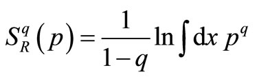
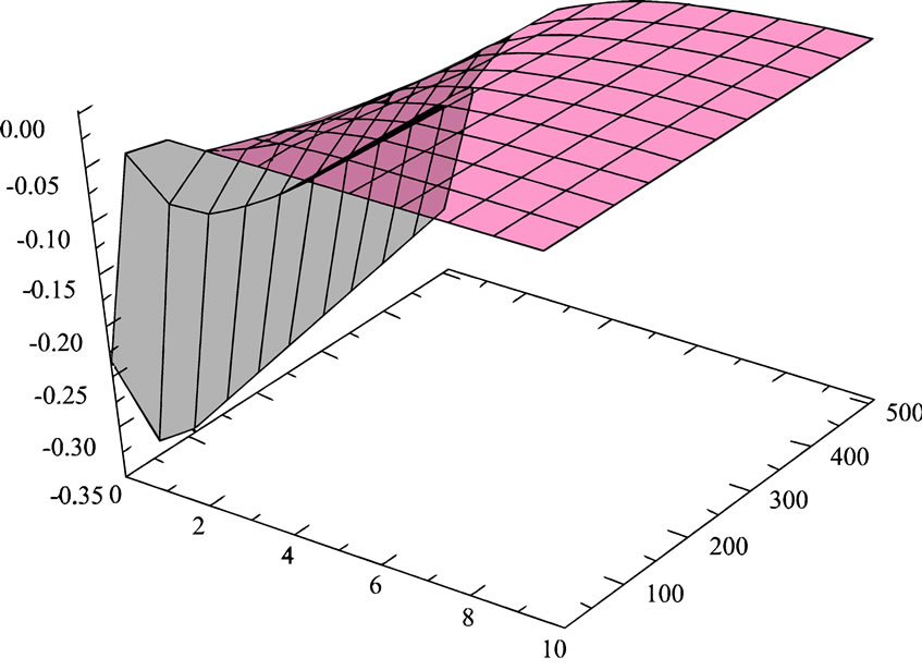
In this section, the non-linear Fokker-Planck equations depending on a category of generalized entropies are studied. The stationary solution of these equations for the Tsallis entropy, Rényi entropy, and Sharma-Mittal entropy has been previously investigated [13-17]. Herein, the Frank method is employed for a large category of entropies. We demonstrate that all the entropies being function of Tsallis entropy can be defined by such solutions. The stationary solution (a) exact solution, (b) approximate solution, and (c) absolute error for the non-linear Fokker-Planck equations are shown in Figure 1. For this purpose, first, it is essential to review the Frank method for the Tsallis entropy. The integral form of Tsallis entropy is as follows:
 (3)
(3)
Regarding Equations (A.1) to (A.4), the equations below are obtained:
 (4)
(4)
provided that .
.
 (5)
(5)
provided that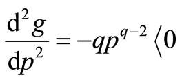 .
.
By considering the linear drift force and inputting the above values to Equation (A.7), we have:
 (6)
(6)
The stationary solution of Equation (6) is the Tsallis distribution function. Instead of directly solving the equation, Equations (A.11) and (A.12) are utilized to obtain the distribution function. Herein, through Equation (A.10),
 (a)
(a)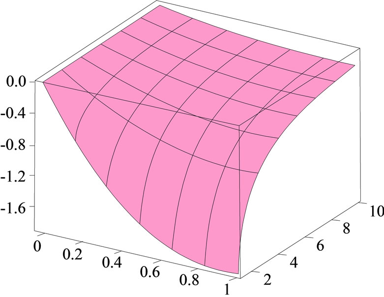 (b)
(b)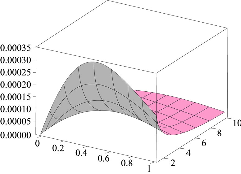 (c)
(c)
Figure 1. The surface shows the stationary solution (a) exact solution; (b) approximate solution, and (c) absolute error for the non-linear Fokker-Planck equations.
h is defined by the following equation:
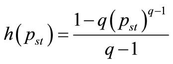 (7)
(7)
 (8)
(8)
Consequently, by using Equation (A.12), we obtain:
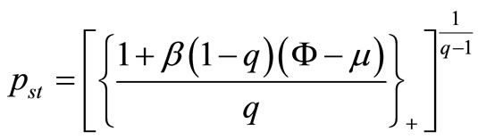 (9)
(9)
 means that the solution will be valid only in cases which the quantity inside the curly brackets is positive. For the linear force
 , the potential Ф is as follows:
 (10)
(10)
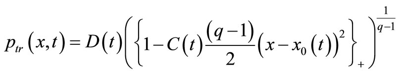
Equation (9) can be rewritten as the form below:
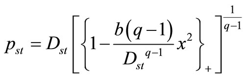 (11)
(11)
In the stationary state, b and the normalization coefficient  are defined as follows:
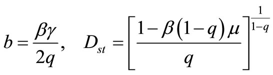 (12)
(12)
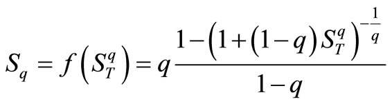
Now, we study a more general state in which the entropy is as a function of Tsallis entropy.
The entropy is defined as  where f is an arbitrary and differentiable function. The distribution function is achieved using Equation (A.8):
 (13)
(13)
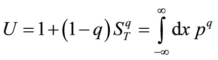
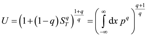
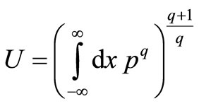
We define a function termed U as the following form:
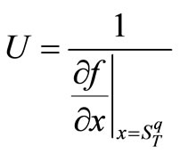 (14)
(14)
Subsequently, Equation (13) can be rewritten as the from below:
 (15)
(15)
Through using Equation (12) and comparing Equations (A.8) with (15), we realize that this general entropy’s distribution function can be achieved by substituting bU for b in Equation (11). Accordingly, this general entropy’s distribution function will be as follows:
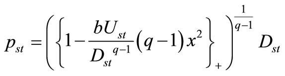 (16)
(16)
The functions b,  , and
, and  are positive. It should be noted that, for the values
 , the distribution function has a cut in
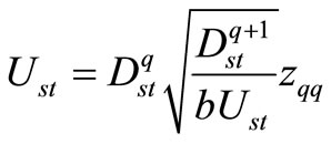
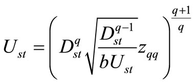
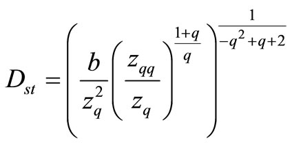
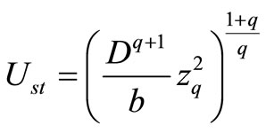
 . To complete the solution, it is sufficient to determine the function Ust and normalization coefficient Dst in relation to each special function
  of
of .
.
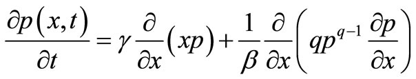
In Equation (6), if βU is substituted for β, its equilibrium-state solution is the above entropy distribution function. The corresponding Fokker-Planck equation will be as follows:
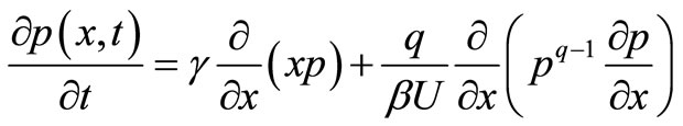 (17)
(17)
For instance, we investigate two entropies being functions of Tsallis entropy, and complete the stationary solution to their Fokker-Planck equation through computing  and
and .
.
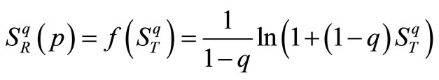
A. First, we consider the Rényi entropy that is defined by the equation below:
 (18)
(18)
 (19)
(19)
Therefore, according to the definition of U in Equation (14), we acquire:
 (20)
(20)
The normalization condition for Equation (16) using the following equation is identical to the definition of function  in Table 1:
 (21)
(21)
Subsequently, we have:
 (22)
(22)
provided that .
.
Roughly similar to the above procedure, the following equation is obtained but through utilizing the definition of function  in Table 1:
 (23)
(23)
provided that .
.
Through inserting Equation (22) into the both sides of Equation (23), we obtain:
 (24)
(24)
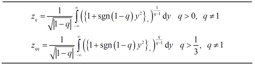
Table 1. The definitions of zq and zqq.
Consequently, the quantities  and
and  are determined by Equations (22) and (24), and the distribution function of Equation (16) is completely defined.
The functions  and
and  can be expressed according to the functions of β and γ [23-31].
In this section, we investigate the entropy defined by the equation below [23-31]. It is a function of Tsallis entropy:
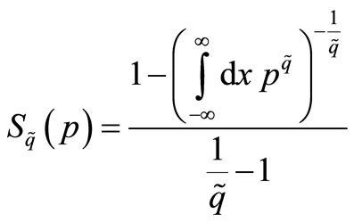 (25)
(25)
 (26)
(26)
The relation between the Tsallis entropy and above entropy can be easily expressed by the function f:
 (27)
(27)
Therefore, based on the definition of U in Equation (14), we have:
 (28)
(28)
The same as the section A, we obtain the following results:
 (29)
(29)
and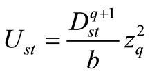 .
.
 (30.1)
 (30.2)
Through inputting Equation (29) to Equation (30.1), we obtain:
 (31)
(31)
By comparing Equations (20) and (28), the function  is determined using Equation (22):
 (32)
(32)
Subsequently, the values of the function U and the normalization coefficient  are determined, and complete the description of stationary solutions to the nonlinear Fokker-Planck equations.
Now, we discuss the limit applied to q in the definition of . For the large x, the integrand in the definition of
 is proportional to
  in
in ; therefore, this integral is divergent. For the large x and
 , the integral is divergent as well, since the integrand is proportional to
 ,
, . Consequently, the limit
  is applied to the entropies which
  is inserted into their distribution functions.
It is important to note that the method proposed in this paper can be solely utilized for the entropies being in the form of . However, this matter does not reduce this method’s significance, because a broad category of entropies can be expressed as a function of Tsallis entropy [23-38]. All the entropies being function of Tsallis entropy are shown in Figure 2.
3. The Time-Dependent Solutions to the Non-Linear Fokker-Planck Equations
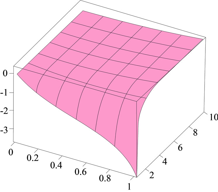
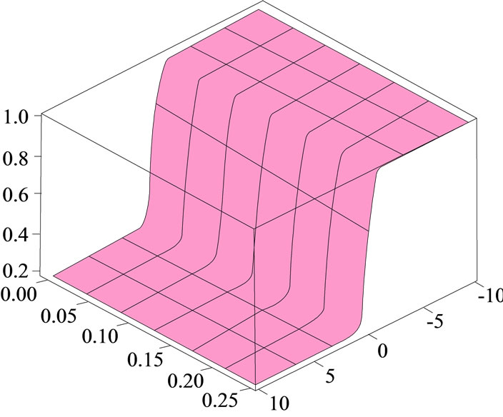
The temporal solution to the entropy-dependent FokkerPlanck Equation (6) has been achieved by Plastino [18- 22]. The same as Plastino’s method, we also assume the temporal solution to the Fokker-Planck Equation (17) as the following form. Equation (17) is related to the entropy .The time-dependent solutions (a) exact solution, (b) approximate solution, and (c) absolute error for the non-linear Fokker-Planck equations are shown in Figure 3. The function U is different in Equations (6) and (17):
 (33)
(33)
The functions  and
and  are positive.
With the aid of the normalization condition and the definitions in Table 1, the relation between
  and
and  is determined:
 (34)
(34)
 (a)
(a)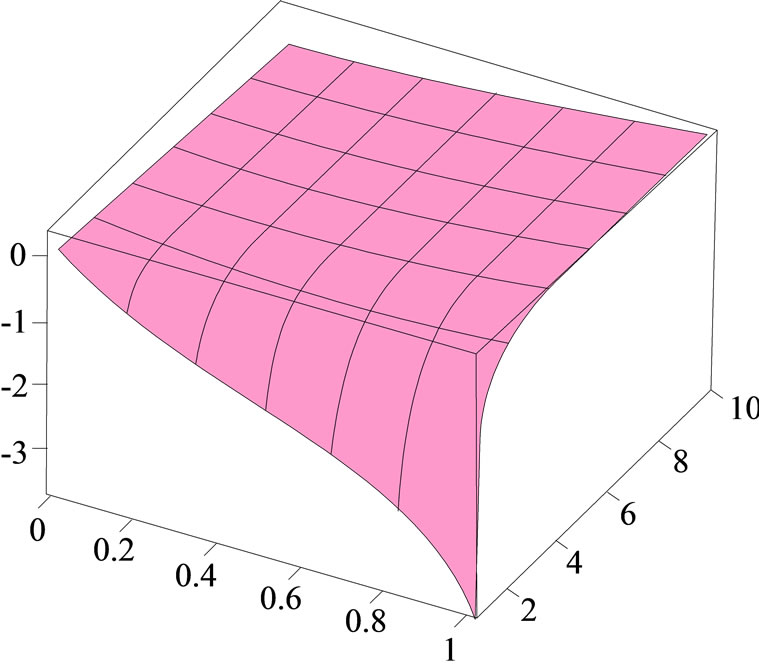 (b)
(b)
Figure 2. The surface shows all the entropies being function of Tsallis entropy.
Through using Equations (33) and (34), inserting them into Equation (17), and then removing the different powers of , the first-order differential equations of
  and
and  can be achieved:
 (35)
(35)
 (36)
(36)
The solution to Equation (35) can be easily obtained:
 (37)
(37)
 (38)
(38)
We input Equation (33) to the definitions of function U for different entropies, and obtain  according to
 . Therefore, without the function
 , Equation (36) can be written and solved in detail for different entropies. For example, Table 2 provides the results of
 (a)
(a)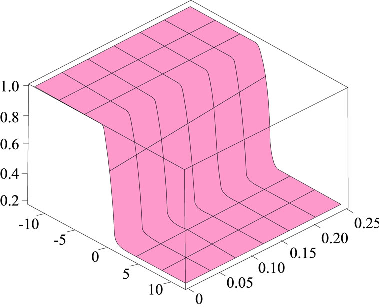 (b)
(b)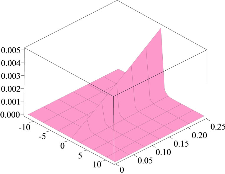 (c)
(c)
Figure 3. The surface shows the time-dependent solutions (a) exact solution, (b) approximate solution, and (c) absolute error for the non-linear Fokker-Planck equations.
three entropies. The approximate solution for Equation (36) for different entropies are shown in Figure 4.
4. Conclusions
In many articles, the generalized Fokker-Planck equations
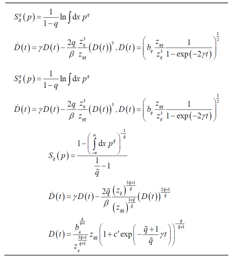
Table 2. Some examples of the differential equation D(t) and their solutions.
 (a)
(a)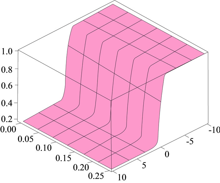 (b)
(b)
Figure 4. The surface shows the approximate solution for Equation (36) for different entropies.
being dependent on Tsallis entropy and some other special entropies are written and solved. The Tsallis entropy and its functions have attracted a great deal of interest owing to the fact that they are desirably consistent with the physical systems with long-term memory, or long-range interactions. As regards the importance of achieving the solutions of Fokker-Planck equations, the following contents can be noted.
In general, the time-dependent distribution function is required to describe a non-equilibrium system. As an example, the diffusing effect is highly interesting in theoretical and empirical terms. The mean square of changes in state variable (variance) is a criterion for dividing the diffusion. If the variance is expressed as  where
where  represents the time,
  ,
,  , and
, and  are respectively called subdiffusion, normal diffusion, and hyperdiffusion. Many examples of each of these three categories are found in nature such as pseudo-polymeric systems, two-dimensional rotational flow, thermal conduction in plasma, population scattering in biological systems and so forth.
5. Acknowledgements
The work described in this paper was fully supported by grants from the Institute for Advanced Studies of Iran. The authors would like to express genuinely and sincerely thanks and appreciated and their gratitude to Institute for Advanced Studies of Iran.
REFERENCES
- C. Tsallis, “Possible Generalization of Boltzmann-Gibbs Statistics,” Journal of Statistical Physics, Vol. 52, No. 1-2, 1988, pp. 479-487. doi:10.1007/BF01016429
- P. H. Chavanis, “Generalized Thermodynamics and Fokker-Planck Equations: Applications to Stellar Dynamics and Two-Dimensional Turbulence,” Physical Review E, Vol. 68, No. 3, 2003, pp. 036108-036127. doi:10.1103/PhysRevE.68.036108
- P. H. Chavanis, “Nonlinear Mean Field Fokker-Planck Equations. Application to the Chemotaxis of Biological Populations,” The European Physical Journal B—Condensed Matter and Complex Systems, Vol. 62, 2008, pp. 179-208.
- P. H. Chavanis, “Generalized Fokker-Planck Equations and Effective Thermodynamics,” Physica A: Statistical Mechanics and Its Applications, Vol. 340, 2004, pp. 57- 65.
- P. H. Chavanis and M. Lemou, “Relaxation of the Distribution Function Tails for Systems Described by Fokker-Planck Equations,” Physical Review E, Vol. 72, No. 6, 2005, pp. 061106-061121. doi:10.1103/PhysRevE.72.061106
- P. H. Chavanis, “Nonlinear Mean-Field Fokker-Planck Equations and Their Applications in Physics, Astrophysics and Biology,” Comptes Rendus Physique, Vol. 7, No. 3, 2006, pp. 318-330. doi:10.1016/j.crhy.2006.01.004
- V. Schwämmle, E. M. F. Curado and F. D. Nobre, “A General Nonlinear Fokker-Planck Equation and Its Associated Entropy,” The European Physical Journal B— Condensed Matter and Complex Systems, Vol. 58, 2007, pp. 159-165.
- V. Schwämmle, F. D. Nobre and E. M. F. Curado, “Consequences of the H Theorem from Nonlinear FokkerPlanck Equations,” Physical Review E, Vol. 76, No. 4, 2007, pp. 041123-041130. doi:10.1103/PhysRevE.76.041123
- V. Schwämmle, E. M. F. Curado and F. D. Nobre, “Dynamics of Normal and Anomalous Diffusion in Nonlinear Fokker-Planck Equations,” The European Physical Journal B—Condensed Matter and Complex Systems, Vol. 70, 2009, pp. 107-116.
- V. Schwämmle, E. M. F. Curado and F. D. Nobre, “Nonlinear Fokker-Planck Equations Related to Standard Thermostatistics,” Complexity, Metastability and Nonextensivity, Vol. 84, 2007, pp. 152-156.
- M. S. Ribeiro, F. D. Nobre and E. M. F. Curado, “Classes of N-Dimensional Nonlinear Fokker-Planck Equations Associated to Tsallis Entropy,” Entropy, Vol. 13, No. 11, 2011, pp. 1928-1944. doi:10.3390/e13111928
- A. M. Scarfone and T. Wada, “Lie Symmetries and Related Group-Invariant Solutions of a Nonlinear FokkerPlanck Equation Based on the Sharma-Taneja-Mittal Entropy,” Brazilian Journal of Physics, Vol. 30, No. 2A, 2009. doi:10.1590/S0103-97332009000400024
- T. D. Frank, A. Daffertshofer, C. E. Peper, P. J. Beek and H. Haken, “Towards a Comprehensive Theory of Brain Activity: Coupled Oscillator Systems under External Forces,” Physica D: Nonlinear Phenomena, Vol. 144, No. 1-2, 2000, pp. 62-86. doi:10.1016/S0167-2789(00)00071-3
- T. D. Frank, A. Daffertshofer and P. J. Beek, “Multivariate Ornstein-Uhlenbeck Processes with Mean-Field Dependent Coefficients: Application to Postural Sway,” Physical Review E, Vol. 63, No. 1, 2000, pp. 011905- 011920. doi:10.1103/PhysRevE.63.011905
- T. D. Frank and A. Daffertshofer, “Exact Time-Dependent Solutions of the Renyi Fokker-Planck Equation and the Fokker-Planck Equations Related to the Entropies Proposed by Sharma and Mittal,” Physica A: Statistical Mechanics and Its Applications, Vol. 285, 2000, pp. 351-366.
- T. D. Frank, “On Nonlinear and Nonextensive Diffusion and the Second Law of Thermodynamics,” Physics Letters A, Vol. 267, No. 5-6, 2000, pp. 298-304. doi:10.1016/S0375-9601(00)00127-4
- A. Daffertshofer, C. E. Peper, T. D. Frank and P. J. Beek, “Spatio-Temporal Patterns of Encephalographic Signals during Polyrhythmic Tapping,” Human Movement Science, Vol. 19, No. 4, 2000, pp. 475-498. doi:10.1016/S0167-9457(00)00032-4
- A.R. Plastino and A. Plastino, “Non-Extensive Statistical Mechanics and Generalized Fokker-Planck Equation,” Physica A: Statistical Mechanics and Its Applications, Vol. 222, 1995, pp. 347-354.
- A. R. Plastino, A. Plastino and H. Vucetich, “A Quantitative Test of Gibbs’ Statistical Mechanics,” Physics Letters A, Vol. 207, No. 1-2, 1995, pp. 42-46. doi:10.1016/0375-9601(95)00640-O
- F. Pennini, A. Plastino and A. R. Plastino, “Tsallis Entropy and Quantal Distribution Functions,” Physics Letters A, Vol. 208, No. 4-6, 1995, pp. 309-314. doi:10.1016/0375-9601(95)00720-1
- A. R. Plastino and A. Plastino, “Fisher Information and Bounds to the Entropy Increase,” Physical Review E, Vol. 52, No. 4, 1995, pp. 4580-4582. doi:10.1103/PhysRevE.52.4580
- M. Portesi, A. Plastino and C. Tsallis, “Nonextensive Thermostatistics Can Yield Apparent Magnetism,” Physical Review E, Vol. 52, 1995, pp. R.3317-R.3320.
- T. D. Frank, “Stochastic Feedback, Nonlinear Families of Markov Processes, and Nonlinear Fokker-Planck Equations,” Physica A: Statistical Mechanics and Its Applications, Vol. 331, 2004, pp. 391-408.
- T. D. Frank, “Analytical Results for Fundamental TimeDelayed Feedback Systems Subjected to Multiplicative Noise,” Physical Review E, Vol. 69, No. 6, 2004, pp. 061104-061114. doi:10.1103/PhysRevE.69.061104
- T. D. Frank, “Fluctuation-Dissipation Theorems for Nonlinear Fokker-Planck Equations of the Desai-Zwanzig Type and Vlasov-Fokker-Planck Equations,” Physics Letters A, Vol. 329, No. 6, 2004, pp. 475-485. doi:10.1016/j.physleta.2004.07.019
- T. D. Frank, “Classical Langevin Equations for the Free Electron Gas and Blackbody Radiation,” Journal of Physics A: Mathematical and General, Vol. 37, No. 11, 2004, p. 3561. doi:10.1088/0305-4470/37/11/001
- T. D. Frank, P. J. Beek and R. Friedrich, “Identifying Noise Sources of Time-Delayed Feedback Systems,” Physics Letters A, Vol. 328, No. 2-3, 2004, pp. 219-224. doi:10.1016/j.physleta.2004.06.012
- T. D. Frank, “Stability Analysis of Stationary States of Mean Field Models Described by Fokker-Planck Equations,” Physica D: Nonlinear Phenomena, Vol. 189, No. 3-4, 2004, pp. 199-218. doi:10.1016/j.physd.2003.08.010
- T. D. Frank, “Complete Description of a Generalized Ornstein-Uhlenbeck Process Related to the Nonextensive Gaussian Entropy,” Physica A: Statistical Mechanics and its Applications, Vol. 340, 2004, pp. 251-256.
- T. D. Frank, “Dynamic Mean Field Models: H-Theorem for Stochastic Processes and Basins of Attraction of Stationary Processes,” Physica D: Nonlinear Phenomena, Vol. 195, No. 3-4, 2004, pp. 229-243. doi:10.1016/j.physd.2004.03.014
- T. D. Frank, “Nonlinear Fokker-Plank Equations,” Springer, Amsterdam, 2004.
- A. M. Mathai and H. J. Haubold, “On Generalized Entropy Measures and Pathways,” Physica A: Statistical Mechanics and Its Applications, Vol. 385, 2007, pp. 493- 500.
- T. D. Frank and A. R. Plastino, “Generalized Thermostatistics Based on the Sharma-Mittal Entropy and Escort Mean Values,” The European Physical Journal B— Condensed Matter and Complex Systems, Vol. 30, 2002, pp. 543-549.
- T. D. Frank, “Generalized Fokker-Planck Equations Derived from Generalized Linear Nonequilibrium Thermodynamics,” Physica A: Statistical Mechanics and Its Applications, Vol. 310, 2002, pp. 397-412.
- T. D. Frank, “On a General Link between Anomalous Diffusion and Nonextensivity,” Journal of Mathematical Physics, Vol. 43, No. 1, 2002, pp. 344-350. doi:10.1063/1.1421062
- T. D. Frank, “Generalized Multivariate Fokker-Planck Equations Derived from Kinetic Transport Theory and Linear Nonequilibrium Thermodynamics,” Physics Letters A, Vol. 305, No. 3-4, 2002, pp. 150-159. doi:10.1016/S0375-9601(02)01446-9
- T. D. Frank, “Interpretation of Lagrange Multipliers of Generalized Maximum-Entropy Distributions,” Physics Letters A, Vol. 299, 2002, pp. 153-158. doi:10.1016/S0375-9601(02)00631-X
- T. D. Frank, A. Daffertshofer and P. J. Beek, “Impacts of Statistical Feedback on the Flexibility-Accuracy TradeOffin Biological Systems,” Journal of Biological Physics, Vol. 28, No. 2-3, 2002, pp. 39-54. doi:10.1023/A:1016256613673
Appendix A: The Generalized Entropies and Dependent Fokker-Planck Equations
The calculations are limited to one dimension in order to simplify. Also, they can be generalized to N dimensions.
The entropies are considered as follows:
 (A.1)
(A.1)
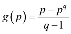
so that  is a well-defined and arbitrary function, and
  is also determined by:
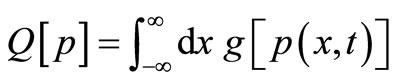 (A.2)
(A.2)
where  is a well-defined function of p which is twice differentiable at least.
The states with zero probability must not affect the entropy; furthermore, the natural systems contain a considerable number of microscopic states; therefore, a state with one probability cannot also affect the entropy; accordingly:
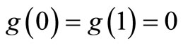 (A.3)
(A.3)
The concavity is one of the entropies’ general conditions. Hence, the entropy should have the following condition [7-12]:
 (A.4)
(A.4)
The non-linear Fokker-Planck equation is defined as follows:
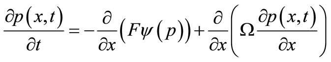 (A.5)
(A.5)
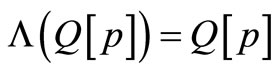
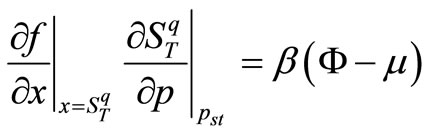
where , and it is the external force resulting from the potential Ф. The parameters Ω and Ψ are the functions of p. Equation (A.7) relates to the entropy through the equation below. Actually, the ratio
  is selected in order that the stationary solution to Equation (A.5) is the entropy distribution function:
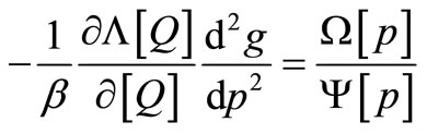 (A.6)
(A.6)
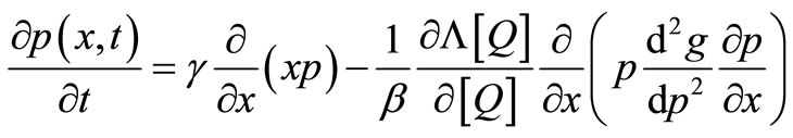
β denotes the inverse temperature. For the linear force  and by selecting
 , Equation (A. 5) is written as the form below:
 (A.7)
(A.7)
In the different references, the Fokker-Planck equation dependent on entropies is investigated in various ways. The above-mentioned issues are comprehensively described in the reference [7-12].
In this section, how to achieve the entropy distribution function of Equation (A.1) is mentioned [32]. The probability distribution function of p is obtained by maximizing the entropy in a canonical ensemble. Therefore in a canonical ensemble, provided the number of particles and the total energy are constant, we obtain:
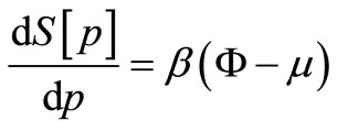 (A.8)
(A.8)
where Ω is the external potential, µ is the system’s chemical potential, and β is the dependent Lagrange multiplier.
Considering the form of entropy in Equation (A.1), we obtain:
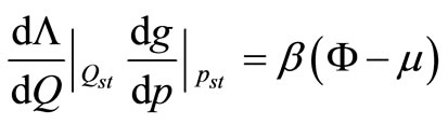 (A.9)
(A.9)
 and
and  indicate the values of these quantities in the equilibrium state and maximum entropy, respectively. The function
  is defined as the form below:
 (A.10)
Therefore:
 (A.11)
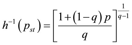
With the aid of the inverse function of h (it means ), we can achieve
  as the following form:
 (A.12)
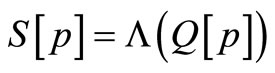
 is the generalized entropy distribution function. The generalized entropies and dependent Fokker-Planck equations are shown in Figure A1.
 (a)
(a) 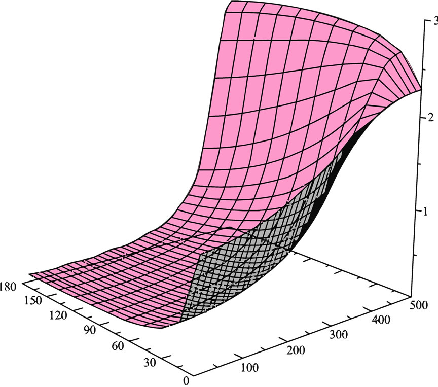 (b)
(b)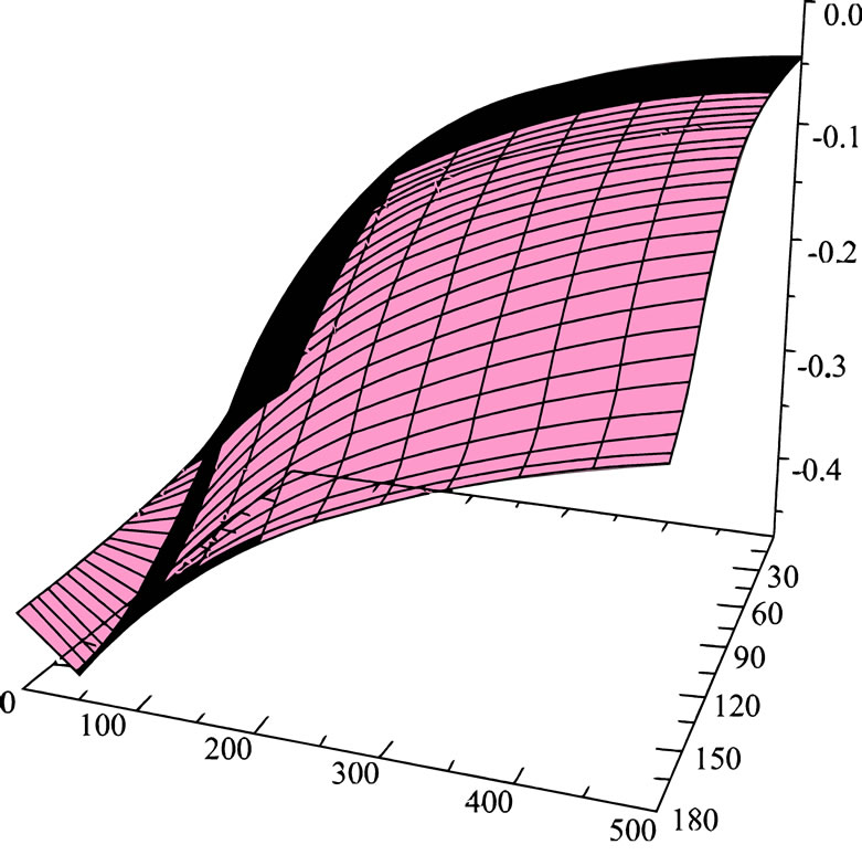 (c)
(c) 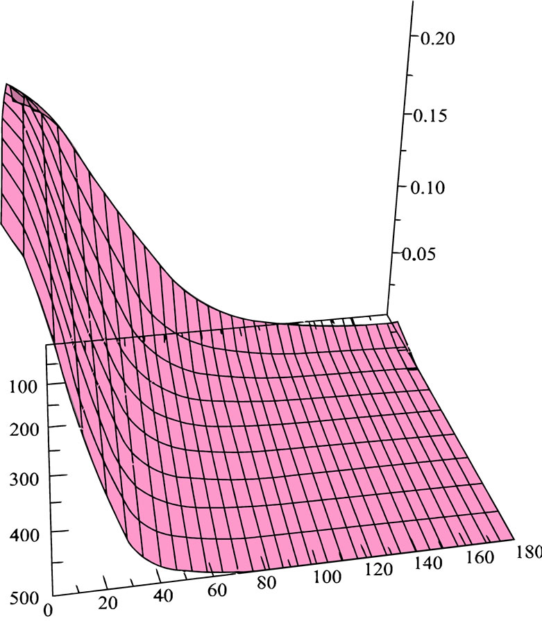 (d)
(d)
Figure A1. The surface shows the generalized entropies and dependent fokker-planck equations.
NOTES
*Corresponding author.