Received 28 October 2015; accepted 19 June 2016; published 22 June 2016

ABSTRACT

Mathematical models based on advanced differential equations are utilized to analyze the glucose-insulin regulatory system, and how it affects the detection of Type I and Type II diabetes. In this paper, we have incorporated several models of prominent mathematicians in this field of work. Three of these models are single time delays, where either there is a time delay of how long it takes insulin produced by the pancreas to take effect, or a delay in the glucose production after the insulin has taken effect on the body. Three other models are two-time delay models, and based on the specific models, the time delay takes place in some sort of insulin production delay or glucose production delay. The intent of this paper is to use these multiple delays to analyze the glucose-insulin regulatory system, and how if it is not properly working at any point, the high risk of diabetes becomes a reality.

Keywords:

Delay Differential Equations, MATLAB, Diabetes, Insulin-Glucose Model

1. Introduction

The human body needs to maintain a level of glucose concentration that is not too high in order for it to function properly. In order for glucose to be produced and utilized, insulin production and utilization must occur. If insulin is not produced, or not enough of it is produced, then proper glucose levels cannot be maintained, which leads to the disease of diabetes. Diabetes mellitus is a condition in which there is too much glucose in our blood. The pancreatic endocrine hormones insulin and glucagon are responsible for regulating and maintaining your body’s glucose concentration level. Insulin is produced in the pancreas, and is released from cells. These cells stimulate the cells to absorb enough glucose from the blood for the fuel or energy that they need. Insulin also stimulates the liver to absorb and store any left-over glucose. Glucagon is released when the glucose concentration level is too low. This stimulates the liver cells to release the left-over glucose into the blood, so cells will have enough energy to carry out their functions. If a person’s blood glucose concentration level is constantly above the normal range for humans, they suffer from the chronic condition, known as diabetes.

There are two type of diabetes. Type I diabetes, or insulin-dependent diabetes, is an autoimmune disease that occurs when the insulin-producing cells in the pancreas are attacked and destroyed by other cells in the body, causing the pancreas to produce little or no insulin at all. The cure for Type I diabetes is to have insulin replacement treatment for the rest of their life. This type of diabetes is known as juvenile diabetes, because it normally develops before the age of 40, often times before then. It is the least common of the two (10%).

Type II, or non-insulin dependent diabetes, is a metabolic disorder which develops when the body can still produce insulin, but not enough, or when the insulin that is produced does not work properly, or better known as insulin resistance. Type II diabetes, is more likely to occur if there is a history of it in your family, and is often associated with obesity. Symptoms for Type II diabetes develop slowly over time, if at all, and occur mostly in people over the age of 40. Life expectancy for the Type I diabetes is reduced by about 15 years, and 10 years for Type II diabetes. If diabetes is left untreated or improperly managed, it can lead to heart disease, blindness, kidney disease, and non-traumatic limb amputations.

Due to these factors and harmful effects of diabetes, many researchers have been motivated to study the glucose-insulin endocrine metabolic regulatory system with hopes to better understand the mechanistic functions and causes of the dysfunction of the metabolic system. Many types of models have been made to better understand the role of the insulin-glucose regulatory system, including ordinary differential equations, and delay differential equation, both of which are included in this paper.

In the glucose-insulin endocrine metabolic regulatory system, the two pancreatic endocrine hormones, insulin and glucagon, are the primary regulatory factors. Numerous in-vivo and in-vitro experiments indicate that insulin secretion consists of two oscillations occurring with different time scales. One is rapid oscillations (5 - 15 min) and the second is ultradian oscillations (50 - 150 min). The mechanisms underlying both types of oscillations are still not fully understood. The rapid oscillations may arise from an intra-pancreatic pacemaker mechanism resulting in periodic secretary bursting of insulin from pancreatic cells. This rapid oscillation is usually super imposed on the slow ultradian oscillation. The ultradian oscillations of insulin secretion are assumed to result from instability in the glucose-insulin endocrine hormones of the metabolic regulatory system.

In this paper, we propose a number of delay differential equation (DDE) models by introducing two and three explicit time delays in order to model the glucose-insulin levels in the metabolic regulatory system. The two and three time delay models not only confirm many experimental observations, but also demonstrate robustness, and produce simulation profiles in better agreement with physiological data. As a result, we suspect that one of the possible causes of ultradian insulin secretion oscillations is the time delay of the insulin secretion simulated by the elevated glucose concentration. Our analysis shows that three time delay model is more accurate than two time delay.

In this paper we use several proposed Delay Differential Equation models (DDE) to show the delays of the metabolic system. We use single delay models in addition of multiple delay models to form a new proposed model combining the theories of the previous models used.

2. Delay Differential Equations

A delay differential equation (DDE) is an equation where the evolution of the system at a certain time, solution t, depends on the state of the system at an earlier time; say. This is distinct from the ordinary differential equation (ODE) where the derivatives depend only on the current value of the independent variable. The solution of the ODEs therefore requires knowledge of not only the current state, but also of the state of a certain time previously.

2.1. Differential Delay Equation Methods

Many approaches of DDE solutions start from the problem in the formulations

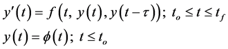(2.1)

The function represents the same physical quantity that evolves overtime. The derivative depends on past values of, represents the initial function, and is the delay term.

The theory of DDEs has become an important area of investigation stimulated by their numerous applications to problem in mechanics, electric, and electronic engineering, medicines, biology, ecology, etc. Since many systems arising from realistic models heavily depend on history (which is characterized by the effect of finite (or infinite) delay on all equations), so there is a need to study partial functional delay differential system with the delay argument; and many evolution process characterized the fact that at certain moments of time they experience a change of state abruptly, this process is subject to short time perturbation whose duration is negligible in comparison with the duration of the process.

There are several approaches to finding numerical solutions to (2.1). These include the direct application of linear multiple step method and Runge-Kutta (4^th order mainly) method for ODEs. If the delay is non-constant, the methods are combined with interpolation.

The first approaches to the numerical solution of DDEs of the above form were characterized by the direct application of formulas for ODEs, called linear multi-step methods. For example, Euler’s forward method, which is

(2.2)

for the same integer.

Beuman’s method ( [1] , Beuman et al., 2003) avoids the need for interpolation in solving the numerical solution of (2.1). To simplify first we consider the case of the constant delay. Then the discontinuity points are. In the first interval, (2.1) has the form

In the second interval and can be defined, so the DDE (2.1) can be written as the two dimensional system of ODEs.

Hence in general, over the interval the DDE (2.1) can be written as the k-dimensional system of ODEs

(2.3)

where,

passing from k to k + 1 means shifting the interval of integration from to , and extending the solution from to by adding the component in the current interval. Therefore, a standard numerical method for solving ODE can be used to solve (2.2), for increasing k, larger system, for each step k, the numerical solution of the k-dimensional system (2.2) is intended to provide an approximate value of to be used as the initial value of the new component in the next step. The process ends when, for some k. So it is necessary to solve a system of ever-increasing dimension and to calculate repeatedly the same pieces of the solution related to the previous intervals. However, due to the presence of the delay argument that is storing and interpolating the computed solution throughout the interval, reducing to a system of ODEs avoids standard complications ( [1] , Beuman et al., 2003).

2.2. An Example of a Delay Differential Equation

Since implies, we have and the differential equation becomes

Therefore,

Using,

Therefore,

In the next subinterval, or, we have

The differential equation becomes

Since,

Therefore,

2.3. Solving Differential Delay Equations in MATLAB

Using the routine dde23 ( [2] , Thompson et al., 2001) in MATLAB, it is easier to solve a large class of delay differential equations (DDE). The problem is restricted to solving systems of equations of the form

for constant delays such that. The equations hold on, which requires the history to be given for. DDE 23 uses explicit Runge-Kutta triple methods in solving Ordinary Differential Equations (ODE), in particular the Runge-Kutta triple BS (2,3), and extends these materials to solve DDEs. A triple of s stages involves three formulas. If you have an approximation to at and wish to compute an approximation at. For, the stages are defined in terms of and

The first formula used in the triple is an approximation used to advance the integration, written in terms of the increment function

(2.4)

The second formula is used only for selection the step size

(2.5)

The third formula is often described as a continuous extension of the first formula, and has the form

(2.6)

The coefficients, , are polynomials in σ, so this represents a polynomial approximation to for. It is assumed that this formula yields the value when and when.

When the delay term is greater than the step size and we have an available approximation to

for all. All the and is an explicit recipe for the

stage and the formulas are explicit, the function is the initial history for. After taking the step to then use (2.6) to define on as.

When the step size is greater than the smallest delay, the “history” term is evaluated in the span of the current step and the formulas are defined implicitly. In this situation the formulas are evaluated with simple iteration. On reading, is defined for. Its definition is extended to and the resulting function is called. A typical stage of simple iteration begins with the approximate solution. The next iteration is computed with the explicit formula

DDE 23 predicts to be the constant for the first step ( [3] , Thompson et al., 2001).

A typical introduction of DDE 23 has the form

sol = DDE23(ddefile, lags, history, tspan);

where ddefile is the name of the function for evaluation the DDE, lags is the constant delays, supplied as an array. history can be specified as the name of a function that evaluates the solution and returns it as a column vector, and tspan is the interval of integration. See ( [4] , Wang et al., 2007) chapter Numerical Results for some examples of using DDE 23 to solve some simple delay differential equation models.

3. Mathematical Models for Diabetes

3.1. Modeling through Ordinary Differential Equations

The insulin-glucose model that is used in this paper was originally developed by Sturis. The purpose of the model was to show the slow oscillations that take place inside of the pancreas and liver, and could give some insight on how they can lead to diabetes if not functioning properly ( [5] , Tolic et al., 2000).

The secretion of insulin in the glucose-insulin endocrine metabolic system occurs in an oscillatory manner over a range of 50 - 150 minutes. Two time delays exist in the time. One is due to the electric action inside of the cells upon glucose stimulation to release insulin. The second time delay represents the delayed effect of insulin on hepatic glucose ( [6] , Li et al., 2006).

The two time delay model of the glucose-insulin regulatory system can be seen in Figure 1.

There are three feedback loops in this model: glucose stimulates pancreatic insulin secretion, insulin stimulates glucose uptake and inhibits hepatic glucose production, and glucose enhances its own uptake. The system also includes two significant time delays: the first is the fact that the physiological action of insulin after the utilization of glucose is correlated with the concentration of insulin. The second is associated with the time lag between the appearance of insulin in the plasma and its inhibitory effect on the hepatic glucose production ( [5] , Tolic et al., 2000).

The model has three main variables: the amount of glucose in the plasma and intercellular space, G, the amount of insulin in the plasma, , and the amount of insulin in the intercellular space,. In addition to the three main variables, there are three others, that represent the above-mentioned delay between insulin in plasma and its effect on the hepatic glucose production ( [5] , Tolic et al., 2000).

The equations describing the dynamics of the model are

(3.1)

(3.2)

(3.3)

(3.4)

(3.5)

(3.6)

Insulin production: Insulin can only be produced by cells in the pancreas. The cell secretion is in in response to the elevated glucose concentration. There are other functions of the cell, however glucose this the most common and important provocation for insulin release. The formula to show the pancreatic insulin production of cells is given as

(3.7)

Insulin degradation and clearance: The liver and the kidney are the primary sites of insulin degradation and clearance. Insulin that is not cleared by the liver or the kidney is eventually removed from other tissues (i.e. muscles). Insulin degradation is process of the kidney and liver that controls insulin action by inactivating and removing the excess of the hormone. Insulin degradation is directly proportional to the insulin concentration. Insulin clearance is the process of regulating the cellular response to the hormone by decreasing insulin availability.

Glucose production: The formation of glucose in the body is caused by two sources. The first is the consumption of carbohydrates, or compounds of carbon, oxygen and hydrogen, that form sugars, starches and fibers. These carbohydrates are absorbed into the bloodstream through hydrolysis. The consumption of carbohydrates takes place through meal ingestion, oral intake (coffee with sugar), etc. The second source of glucose production is the liver. When level of glucose concentration in the bloodstream drops, the cells stop releasing insulin. However, cells, also released by the pancreas begin to release another hormone, glucagon. When glucagon is released it takes control of metabolic pathways (or a sequence of chemical reactions undergone by a compound or class of compounds in a living organism―definition off internet) in the liver, and forces the liver to release glucose.

Glucose Utilization: Glucose utilization, like glucose production consists of two parts, insulin-independent utilization, and insulin-dependent utilization. Insulin-independent glucose consumers are the brain and nerve cells. This glucose intake of the brain and nerve cells is given as

(3.8)

This function represents the dependency on the glucose concentration alone ( [6] , Li et al., 2006). Glucose utilization for muscles and fat tissues depend not only on glucose concentrations levels, but also insulin concentration levels. The shows the glucose dependent term describing glucose utilization

(3.9)

The insulin dependent term is given as

(3.10)

Production of glucose controlled by insulin concentration (I) is stated as hepatic glucose production. In healthy people the pancreas has the ability to constantly measure levels of glucose in the bloodstream. The pancreas then responds to the glucose levels and releases a certain amount of insulin to counteract the glucose intake. The formula to show the above reaction is

(3.11)

3.2. Analysis of Insulin Glucose Feedback Model

In order to fully understand certain feature of the model, the insulin-glucose feedback model has been simplified. The simplified model has two important properties: it is analytically tractable, and it shows the same main characteristics as the original model (i.e. self-sustained oscillations and values of the state variables in the same range as the original model) ( [5] , Tolic et al., 2000).

The function is approximated with a constant and the function by a first-order polynomial. The function is also well approximated by a first-order polynomial in the range of obtained values of intercellular insulin. The function shows significantly greater variation in its second derivative than all the other functions, in the range of glucose and insulin concentration. For values of I in the range 65 - 115 mU in changes from concave to convex, and is well approximated by a third-order polynomial.

The function is replaced with the first-order Taylor expansion around the mean value of G, with a constant, with the first-order expansion around the mean value of I, and with the third- order expansion around the mean value of I. Note that the mean values were obtained by a simulation of glucose infusion at the rate of 216 mg∙min⁻¹ using the original model ( [5] , Tolic et al., 2000) and Table 1 and Table 2. The

standard model to for the detection of diabetes without delay is studied and analyzed. It is well accepted, reasonable and reliable model, refer [7] .

The simplified model is

(3.12)

(3.13)

(3.14)

(3.15)

(3.16)

(3.17)

The time evolution of plasma glucose and insulin concentration that result from the simplified model does not differ significantly from the results of the original model.

In the simulation of an exogenous insulin infusion, equation, , was replaced by

(3.18)

where m = 21 mU/min. A was set to zero for the constant infusion and to 0.3 for the oscillatory infusion. The period T = 120 min. Since the glucose infusion rate in the experiments equals 420 mg/min, using Table 1 and Table 2 (experimental data). The parameter p in Equation (3.14) was set to 285 mg/min to compensate for the difference between the rate of the glucose infusion of 420 and 216 mg/min ( [5] , Tolic et al., 2000).

From an exact solution of the two first order differential equations (3.13) and (3.18), the numerical solutions to (3.15)-(3.17) were computed. For large t, the solutions are periodic functions with period T and may be expressed in the form

(3.19)

The only equation in the simplified model with non-linear terms is Equation (3.14). It can be expressed in the form

(3.20)

where

(3.21)

and

(3.22)

Equation (20) has the general solution

(3.23)

where

(3.24)

(3.25)

and

(3.26)

3.3. Modeling through Delay Differential Equations

In section 3.1 we have discussed the dynamics of the insulin-glucose feedback system through Equations (1)-(6). The hepatic glucose production time delay is stimulated by introducing three auxiliary variables, , which is caused the third order delay. We demonstrate how the auxiliary variables stimulate the time delay as follows: For the sake of convenience we would like to assume the first order delay (i.e.).

Then

When

Using Taylor’s Series Expansion for the function of one variable, we get

I: Explicit Single Time Delay Differential Equation Model

In [8] , Engleborghs et al. (2001) replaced the auxiliary variables, and introduced a single time delay in the Negative Loop Model and proposed the flowing DDE Model

where the functions, and their parameters are assumed to be the same as those in the model (Section 3.1.1). G(t) is the amount of glucose, and are the amounts of insulin in the plasma and the intercellular space, respectively. is the plasma insulin distribution volume, is the effective volume of the intercellular space, E is the diffusion transfer rate, and are the insulin degradation time constants in the plasma and intercellular space, respectively. indicates the (exogenous)glucose supply rate to the plasma, and are three auxiliary variables associated with certain delays of the insulin on the hepatic glucose production in time. The positive constant delay mimics the hepatic glucose production delay.

This model consists of two negative feedback loops, describing the effects of insulin on glucose utilization and glucose production, respectively. Both loops include the stimulatory effect of glucose on insulin secretion. The model mimics the delayed insulin-dependent glucose uptake by splitting the insulin into two separate compartments, plasma and interstitial space. The hepatic glucose production time delay is simulated by introducing three variables (third order delay).

Unfortunately, this model overlooked the time delay from glucose stimulated insulin release to the delayed insulin-dependent glucose uptake. Due to the complex chemical reactions of the cells, it takes a few minutes (5 - 15 mins) for the insulin being ready to help cells utilizing glucose after the plasma glucose concentration level is elevate. As confirmed by, Sturis et al. (1995) [9] , Tolic (2000) [5] , the effects of time delay are significant (Li et al., 2006) [6] .

II. Single Time Delay Proposed by Drozdov and Khanina (1995) [10]

The rate of insulin secretion is assumed to depend only on the glucose concentration. is as follows

The numerator in the right-hand side of the numerator in characterizes the rate of insulin secretion for very large concentrations of glucose. Parameters a and b are determined using experimental data (let a = 5.21 and b = −0.03).

The function is suggested as

The rate of glucose production is assumed to depend only on the insulin concentration, but at the moment, where is a delay in glucose production. The parameter lies in the interval from a few minutes to an hour. The function is proposed as

The delay in this proposed model is a delay in the term (term in other models). The rate of glucose production in the term is assumed to only depend on the insulin concentration, at the moment, where is a delay in glucose production, which affects the amount of glucose produced by the liver. ( [10] , Drozdov et al., 1995).

The model is as follows

where (Volume of plasma) = 3, (Volume of interstitial liquid) = 11, (Volume of the glucose compartment) = 10

III: Explicit Two Time Delay Differential Equation Model

This is a single delay DDE model used for insulin therapies for both Type I and Type II diabetes mellitus and insulin degregation rate assumes Michaelis-Menten kinetics. The model equations proposed by Wang, Li, and Kuang (2009) [11] , is as follows

The major analytical results of this model were to obtain a sufficient condition for global asymptotical stability induced by a Liapunov function with the hepatic glucose production time delay satisfying the cases when and. This result has the following consequences: 1) If the hepatic glucose production time delay, , and the insulin transfer time between the plasma and interstitial compartments, and, are sufficiently small, then the solution converges to a steady state. 2) If the hepatic glucose production value, , is very small, the oscillation will not be sustained.

For Type I diabetes, b = 0, (means no insulin is secreted from the pancreas). For Type IIdiabetes,. In this approach, we keep one explicit time delay as that in the two time delay model and, but mimic the hepatic glucose production time delay by variable chain as in the model in Section 3.1.1. ( [11] , Wang et al., 2009).

IV: Alternative Explicit Two Time Delay Differential Equation Model (Insulin Therapies Related Model)

The idea of insulin therapy is to mimic the normal reaction of the beta cells in the pancreas when they are stimulated by an increase in glucose concentration of the blood, for example after meal ingestion. Numerous experiences have demonstrated that insulin is released from beta cells in two oscillatory models: pulsatile oscillations and ultradin oscillations. Insulin therapies must mimic the insulin secretion at these two time scales and are normally introduced based on clinical experiences, although mathematical models have been proposed for some specific situations ( [4] , Wang et al., 2007).

In the paper by Wang, the following generic model is put forward to simulate the pancreatic insulin secretion with insulin infusion after blood glucose concentration increases for Type I diabetes. We model the effect of time delay t₂ in glucose utilization by and. This results in the following alternative model with two explicit delays.

The notations in models (III) and (IV) are the same as the models discussed previously. Data are used from Table 1 and Table 2 to set up the MATLAB codes.

V: Alternative Explicit Two Time Delay Differential Equation Model (Two-Time Delay Model proposed by Li, Kuang, Mason (2006)) [6] .

Li, Kuang, and Mason consider two time delays: and. The first, , is to denote the total time delay form the time that the glucose concentration level is elevated to the moment that the insulin has been transported to the interstitial space and becomes “remote insulin”. Therefore insulin secretion can be approximated by with time delay.

The second time delay, , has to do with the delay of effect of hepatic glucose production measured from the time that the insulin has become “remote insulin” to the moment that a significant change of hepatic glucose production occurs. in the model represents glucose utilization delay. The model is as follows ( [6] , Li et al., 2006)

This model suggests that the time delay from insulin secretion stimulated by glucose to the insulin becoming “remote insulin” is not negligible; especially the delay of insulin secretion triggered by elevated glucose. Therefore, we suspect that one of the possible causes of ultradian insulin secretion oscillations is the time delay of the insulin secretion stimulated by the elevated glucose concentration.

In this two time delay model, denotes the total delay from the time that the glucose concentration level is elevated to the moment that the insulin has been transferred to the interstitial space, thus becoming ‘remote insulin’. has to do with the delay of hepatic glucose production measured from the time that insulin has become ‘remote insulin’ to the moment that a significant change of hepatic glucose production occurs. is the glucose infusion rate; is the insulin clearance rate. Functions are defined previously.

Based on our numerical simulations and analysis, we suspect that time total time delay, , is critically responsible for the oscillation. The total time delay is measured from the moment that the glucose concentration level starts to increase to the moment that the insulin has been transported to the interstitial space.

VI: Another Alternative Two Time Delay Differential Equation Model, (Palumbo, Panunzi, DeGaetano [2004]) [12]

To our knowledge, there are no mathematical models considering cell activity in the form of DDEs. Our aim is to describe the activity of cell through the flowing two time delay DDE model.

where is the apparent delay with which the pancreas varies secondary insulin release in response to varying plasma glucose concentration. is the delay with which insulin acts in stimulating glucose uptake by peripheral tissues ( [12] , Palumbo et al., 2004). This model is very similar to the one given in (V).

There are two possibilities of delay of insulin release by the pancreas in response to variation of glucose concentration in plasma: (1), (2)

This model describes the dynamics of the glucose-insulin feedback system which involves an equation for the number of cells. Additionally, it provides a description of the mechanisms that link glucose metabolism to changes in the electrical activity of cell that induces insulin secretion. Codes for the numerical simulations of this model are as follows:

VII: Multiple Time Delay Model

The final model, which has not been considered, is a multiple delay differential equation, made from combinations of the previous four models given. The model is as follows:

This model is made up from all of the previous sections, taking common delays from each and making one model out of the previous five, and adding one additional delay in. The two time delays in come from the model proposed by Wang, Li, and Kuang in 2007 (Section IV) [4] . Similarly in 2006, Li, Kuang and Mason [6] , made an earlier model (Section V) that proposed the time delay in in and the time delay in. We connected the two proposed models to form the basis for our final model. The time delays in and are also related form the model proposed by Palumbo, Panunzi, and DeGaetano in 2004 (Section VI) [12] . The last three equations with the time delay in the equation, were taken from the model proposed by Drozdov and Khanina ( [10] , Drozdov et al., 1995).

This function represents all the delays we have presented so far in this paper. The time delays in the function and_. In this equation the is seen in the, or the glucose production controlled by insulin concentration, and represents the hepatic glucose production delay. The seen in the, or the insulin- dependent glucose uptake (dependent upon glucose because multiplied by), is the time delay for the insulin-dependent glucose utilization by the cells ( [4] , Wang et al., 2007).

The delay in the term is represented by, which is the total time delay form the time that the glucose concentration level is elevated to the moment that the insulin has been transported to the interstitial space and becomes “remote insulin” as stated in Section V. This delay can be added to our model, because the time delay is shared between the model in Section IV and Section V. The last delay in our system is the delay in the term, given by Drozdov and Khanina ( [10] , Drozdov et al., 1995). This delay represents the delay in glucose production, which affects the amount of glucose produced by the liver.

Remark: The parameter values assumed in Figures 1-3 are experimental values. Such values may have significant effects on the results studied in this paper.

Summary: In this paper, we studied delay differential equation (DDE) models by introducing two and three explicit time delays and model the glucose-insulin endocrine metabolic regulatory system. The three-time delay model not only confirms many exciting experimental observations, but also demonstrates robustness, and produces simulation profiles in better agreement with observed data. As a result, we suspect that one of the possible causes of ultradian insulin secretion oscillations is the time delay of the insulin secretion simulated by the elevated glucose concentration. Like the two-time delay models, three-time delay models can also be generalized to get more accuracy in the detection of diabetes.

Acknowledgements

We are thankful to Dr. Roger Thelwell (James Madison University, VA) for working with us throughout the process to set up the MATLAB codes.

Cite this paper

Dimplekumar Chalishajar,David H. Geary,Geoffrey Cox, (2016) Review Study of Detection of Diabetes Models through Delay Differential Equations. Applied Mathematics,07,1087-1102. doi: 10.4236/am.2016.710097

References

- 1. Beuman, A. and Zennaro, M. (2003) Numerical Methods for Delay Differential Equations. Oxford University Press, NY, USA.
- 2. Thompson, S. and Shampine, L.F. Solving Delay Differential Equations with dde23.
http://www.radford.edu/thompson/webddes/tutorial - 3. Thompson, S. and Shampine, L.F. (2001) Solving Delay Differential Equations in MATLAB. Applied Numerical Mathematics, 37, 441-458.
- 4. Wang, H.Y., Li, J.X. and Kuang, Y. (2007) Mathematical Modeling & Qualitative Analysis of Insulin Therapies. Mathematical Biosciences, 210, 17-33.
http://dx.doi.org/10.1016/j.mbs.2007.05.008 - 5. Tolic, I.M., Mosekilde, E. and Sturis, J. (2000) Modeling the Insulin-Glucose Feeback System: The Significance of Pulsatile Insulin Secretion. Journal of Theoretical Biology, 207, 361-375.
http://dx.doi.org/10.1006/jtbi.2000.2180 - 6. Li, J.X., Kuang, Y. and Mason, C.C. (2006) Modeling the Glucose-insulin Regulatory System and Ultradin Insulin Secretory Oscillations with Two Explicit Time Delays. Journal of Theoretical Biology, 242, 722-735.
http://dx.doi.org/10.1016/j.jtbi.2006.04.002 - 7. Chalishajar, D. and Stanford, A. (2014) Mathematical Analysis of Insulin-Glucose Feedback System of Diabetes. International Journal of Engineering and Applied Sciences, 5, 36-58.
- 8. Englrborgh, K., Lemaire, V., Belair, J. and Roose, D. (2001) Numerical Bifurcation Analysis of Delay Differential Equations Arising from Physiological Modeling. Journal of Mathematical Biology, 42, 361-385.
http://dx.doi.org/10.1007/s002850000072 - 9. Sturis, J., Scheen, A.J., Leproult, R., Polonsky, J.S. and Van Cauter, E. (1995) 24-Hours Glucose Profilesduring Continuous or Oscillatory Insulin Infusion. Journal of Clinical Investigation, 95, 1464-1471.
http://dx.doi.org/10.1172/JCI117817 - 10. Drozdov, A. and Khanina, H. (1995) A Model for Ultradin Oscillations of Insulin and Glucose. Mathematical and Computer Modelling, 22, 23-38.
http://dx.doi.org/10.1016/0895-7177(95)00108-E - 11. Wang, H.Y., Li, J.X. and Kuang, Y. (2009) Enhanced Modeling of the Glucose-Insulin System and Its Applications in Insulin Therapies. Journal of Biological Dynamics, 3, 22-38.
http://dx.doi.org/10.1080/17513750802101927 - 12. Palumbo, P., Panunzi, S. and De Gaetano, A. (2004) Qualitative Behavior of a Family of Delay-Differential Models of the Glucose-Insulin System. Istituto Di Analisi Dei Sistemi Ed Informatica, 620, 3-28.