ABSTRACT

We start with analyzing stochastic dependence in a classic bivariate normal density framework. We focus on the way the conditional density of one of the random variables depends on realizations of the other. In the bivariate normal case this dependence takes the form of a parameter (here the “expected value”) of one probability density depending continuously (here linearly) on realizations of the other random variable. The point is, that such a pattern does not need to be restricted to that classical case of the bivariate normal. We show that this paradigm can be generalized and viewed in ways that allows one to extend it far beyond the bivariate or multivariate normal probability distributions class.

Keywords:Multivariate Probability Distributions, Stochastic Dependence Paradigms, Multivariate Gaussian Distributions, Parameter Dependence Method of Construction, Conditioning, Stress, Biomedical Applications

1. Introduction

This paper can be viewed as an extension of our previous work (Filus and Filus [1] ) on the bivariate Gaussian pdf structure’s genesis of wide classes of newly constructed bivariate probability distributions. These distributions we constructed in our papers since 2000 up to recently (see, Filus and Filus [1] -[6] , also see Kotz, Balakrishnan and Johnson [7] pp. 217-218). Here, our explanations concerning the relation of our models to the bivariate normal were modified and we extended the topic to higher dimensional models and to the relation between our “parameter dependence method” of models construction and the multivariate normal paradigm.

It is a well-known fact that among existing multivariate probability distributions, there are no more than a few classes that are widely and successfully applied in practical stochastic modeling procedures. Typically, the underlying random variables are assumed to be independent or having an “approximately Gaussian” bivariate or multivariate distribution. The normality often is assumed even when corresponding data hardly agree with that mathematical model (showing asymmetry, for example). On the other hand, from all the multivariate distributions used in applications, the normal seems to be “the best”. The reason for this is that the Gaussian models catch the stochastic relationship (mainly by a regression function) between its marginal random variables in the most natural way. We first analyze and interpret the specific way the multivariate normal density of the random vector relates to the marginal quantities. Next we extend the “Gaussian pattern” to more general classes of bivariate and multivariate distributions including cases with non-Gaussian marginals. First of all we show that the common “mechanism” of the stochastic dependences both in the Gaussian distributions structure and the structure of the distributions we define, relies on the same way of conditioning. Namely, in all the considered cases, the conditional density of one random variable, say, , given realizations, say, , of the marginal random variables can be obtained by setting (often arbitrarily) an “initially constant” parameter, say, q_j of the density of X_j to be any continuous function of the realizations. In this way the conditional pdf of X_j, given is defined, which stands for the “source” of the stochastic dependences.

Pursuing this method successively for we always arrive at a unique model. This manner, however, is characteristic for the m-variate normal where we turn an “original” normal N(m_j, σ_j) density of X_j into the conditional density by setting a new value of the “affected old parameter m_j” to be the following (linear regression) function:. Our main contribution is to generalize the latter function to any, not necessarily linear, function and consider not only the parameter m_j but also any other parameter of any probability density to define the corresponding conditional distributions. This is the essence of the socalled parameter dependence method. Specifically in this paper, our task will be showing more closely relation of this method to the multivariate Gaussian model construction.

In Section 2, we analyze the stochastic dependences between marginal random variables of the bivariate normal in order to point out the original version of the parameter dependence pattern next extending to other constructed bivariate probability densities. The explanation as well as the example of applications of the bivariate normal is different from that in Filus and Filus [1] . In Section 3 we present the extension of the bivariate normal pdf to the bivariate FF-normal (formerly called “pseudonormal”). In Section 4 we apply the parameter dependence method to construct the bivariate FF-Weibull (formerly “pseudo-Weibull”) density in reliability framework of joint density of parallel system components life times. Comparison with other, similar, methods in the literature is presented in Section 5. In Section 6 we extend the constructions from bivariate to multivariate probability densities, first showing their relation with the multivariate normal dependences structure. Examples of the construction of multivariate FF-normal and multivariate FF-exponential (“pseudo-exponential”) densities are given.

In Section 7, we point out that the “method of parameter dependence” is used in some more areas of reliability theory for different situations than we are considering. This is a part of the accelerated life testing theory where the dependence of life time distribution’s parameter from a given (high) stress is investigated.

Another (fairly new) area is the “load optimization theory” sometimes associated with the load sharing phenomena analysis that we sketch in Subsection 7.2. The differences between these approaches and our theory are pointed out in 7.2.

2. The Bivariate Normal Case

We start with the following situation. Suppose the normally distributed random variable X₂ describes an attribute of a physical or biological object, say u. Consider the (stochastic) behavior of the object u in two distinct “physical” situations. In the first situation, u is exposed to some random stress whose magnitude is described by a normally distributed random variable X₁. In the second situation we assume there is no such a stress present or the stress takes on a fixed predetermined value. The usual task here is to determine the joint distribution of X₁, X₂. Let the densities of X₁, X₂ be normal, i.e., ,. [It is clear that we must assume that the value (m₂ – kσ₂) is positive for at least k = 3, in order to assure approximate positivity of the normal life-time X₂].

2.1. Simplified Biomedical Example

Imagine the following fictitious experiment whose goal is to establish the possible stochastic impact of a medication’s dose change on some cancer treatment results. Suppose a person of a certain fixed age, was diagnosed with a kind of cancer. Assume that one of the significant characteristics of that kind of cancer is a tumor with a size X₂. During a given time period T after the patient was diagnosed, a specific medication was administered. Also suppose that this medication was routinely administered in the past, and that the average dose is estimated (or fixed) to be m₁ milligrams per kilo of weight daily. Assume that, originally, the known (either measured or estimated) average size of the tumor is, say, m₂ millimeters and after the period T of treatment the tumor size X₂ is measured again and its negative or positive increment is statistcally confronted with the dose X₁ of the medication administered.

We assume that the goal of the underlying experiment is to make a prediction on effect of the treatment when the dose is changed from its “original level” to a level. Randomness of the doze X₁ may be justified when only “historical data” are analyzed and then extrapolated for a larger population of cases not yet recorded. In the case of extrapolation of historical data for a larger population we assume that the only information one possess on the applied in the past dose X₁ is its probability distribution, which is the Gaussian with given values for both the parameters m₁, σ₁. Also, for the tumor size X₂ (after the treatment) is assumed to be a random variable having a normal density, where is the value of the tumor “increment” under the treatment characterized by the dose level m₁. For any other applied doze X₁ = x₁ the, associated with a single patient, value (x₁ – m₁) statistically affects the change in the tumor size X₂ – m₂ i.e., the treatment result. The word “statistically” here means that the impact of a nonzero quantity (x₁ – m₁) (“the dose is not the standard one”) on the (former) probability density N(m₂, σ₂) of the tumor size X₂ realizes through affecting the value of the mean m₂ rather than directly affecting the numerical value x₂ of X₂.

If we were interested in finding the joint probability distribution of X₁, X₂ it is enough to determine the conditional density g₂(x₂|x₁) of X₂|X₁, since the marginal density of X₁ is not changing. 

In accordance with the “linear regression rule”, the dependence of the (new) expected value (so new probability density) of the tumor size X₂ on the event X₁ = x₁, is determined by the familiar functional relationship:

(1)

where a = r(σ₂/σ₁) and r is the (linear) correlation coefficient of the variables X₁, X₂ .

This approach directly leads to the determination of the conditional density of the random variable X₂ given any realization X₁ = x₁. It is a well-known fact that the conditional density g₂(x₂|x₁) is, again, normal and

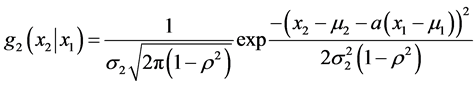, (2)

i.e., the density in x₂.

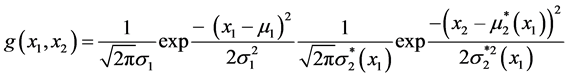
The joint density g(x₁,x₂) of the random variables X₁, X₂ is given by the usual arithmetic product g₂(x₂|x₁)g₁(x₁) .

2.2. Remark

In the example above, one can reinterpret the “response random variable” X₂ to be for example the patient’s “residual life-time”, or blood pressure, or level of some important chemical in the blood (such as cholesterol). In such cases the mathematics of the problem would remain the same.     

Note the obvious fact that the tumor size X₂ does not have a physical influence on the medication dose X₁ so that the original marginal pdf g₁(x₁) remains the same. However, the stochastic dependence between X₁, X₂ is mutual, since, in general, g₁(x₁|x₂) ≠ g₁(x₁).

It is well known that the actual problem with the bivariate normal density construction is to get to the conditional density (2), which fully represents the underlying stochastic dependence of random variable X₂ on X₁.

Our claim is that the above paradigm for the stochastic dependence (characteristic for the bivariate Gaussians) can be extended to other classes of bivariate and multivariate distributions (see Filus and Filus [3] [4] ).

3. The FF-Normal (Pseudonormal) Extension

Historically, people relied on the nice symmetry in the stochastic dependence of X₁ and X₂ when using their joint bivariate normal distribution. This kind of symmetry (i.e., both marginal and both conditional distributions are normal and both sides regression functions are linear) can only be achieved with the linear regression functions as described above (1). However, are linear regression functions really the only functions that one can successfully apply within this framework? Assuming that the function m₂(X₁) is any continuous function in X₁, one obtains a wide and interesting extension of the class of bivariate normal densities. We called this class FF-normal (previously named “pseudonormal”, see [2] and also [7] ). In this case the parameter σ₂ can as well become a continuous function of the stress X₁ (X₁ may have a “stress” interpretation in a very wide sense). This stress may change the parameter σ₂ of the (normal) density of, say, the “life-time” X₂ into another value that depends on the particular realization x₁ of the random variable X₁. The price for such a wide generalization is loss of the, mentioned above, symmetry (the marginal of X₂ ceases to be normal) but the gains are considerable. Anyway, the bivariate normal remains to be a special cases of the FF-normals.

With the bivariate FF-normal densities of (X₁, X₂) we can use general continuous m₂(x₁) and σ₂(x₁) functions, and, performing similar calculations as above, we find, rather surprisingly, that g₂(x₂|x₁) is once more a regular normal density in x₂.

Consider now the following situation with a bivariate FF-normal distribution in which the “physical” interpretation of the underlying random variables can now be more general than above. Let u₁, u₂ be two objects (or phenomena) which are characterized by the random variables X₁, X₂ respectively. If the objects are physically separated then the random variables X₁, X₂ are assumed to be independent, having normal pdfs and respectively. When the objects physically interact (or rather only u₁ physically impacts u₂), then the corresponding joint FF-normal density g(x₁, x₂) of the random vector (X₁, X₂) is given by the usual product formula:

with the invariant marginal density.

For the conditional density of X₂|x₁ we have:.

The functions are “formed” from the “no-stress” parameters m₂, σ₂ of X₂’s density.

More explicitly, one obtains the bivariate FF-normal pdf in the form:

where is the (in general, nonlinear) “regression function”, and is the conditional variance obtained from the “previous” variance.

In particular, one may consider the “nonlinear regression function”

with arbitrary real parameters and A,.

Realize that in the case A = 0 and we obtain the regular bivariate Gaussian density. The coefficient A of the term may be considered as a nonlinear “correction” of the regular Gaussian (linear) regression. The main purpose of that correction is to enhance the accuracy in various modeling procedures. For some type of asymmetric data, especially interesting may be the “non-symmetric” “quadratic” case n = 2.

Equally important is the “symmetric” “cubic” case when n = 3. Also interesting is the case where a^* = 0 and A ≠ 0. Here, the linear correlation coefficient is zero, while the (nonlinear) dependence may be quite “heavy”. Another interesting case (which may be combined with those above) is when we choose the standard deviation function as belonging to the “parametric class” of “quadratic functions” defined by with k positive real. It is rather obvious that the idea of the construction of bivariate normal (and FF-normal as well) can be extended to other probability distributions such as exponential, gamma, Weibull, lognormal, etc.

Generally speaking, the essence of the construction method is that for any pair of (“initially independent”) random variables X₁ and X₂ with given probability densities and respectively, one can simply “declare” some parameter (or a vector parameter), say Θ, of the density to be dependent on the values of the other random variable X₁. This means that when X₁ = x₁ we may assume that is the “affected by x₁” distribution of the random variable X₂ (given the event X₁ = x₁ occurred, with probability density g₁(x₁) ).

Then the joint density of the pair (X₁, X₂) is always.

This situation is especially natural if we consider X₂ to be the life-time of an object and X₁ is the stress put on it.

Roughly, one can say that the construction method of bivariate distributions, presented above is an extension of the method used in the construction of the bivariate normal.

4. Reliability Example

Consider a 2-component (say u₁, u₂) parallel system reliability setting in which X₁, X₂ represent the components’ life-times (see Barlow and Proschan [8] ). We start with the situation where the system’s components act separately. We call that pattern the “laboratory conditions”. In this latter case the components are physically separated and consequently their life-times (represented by the, statistically estimated, “baseline probability densities” g₁(x₁) and g₂(x₂) respectively), are stochastically independent. When the two components are installed into the system, they start to interact. Assume that during that interaction some irregularities in the work of component u₁ cause corresponding changes in u₂’s inner physical structure. This increases the hazard rate of that physically affected component u₂. Such physical phenomena are then “responsible” for the occurrence of stochastic dependence in the “in-system” component life-times X₁ and X₂.

One can also imagine this situation as follows. During the two components’ “in-system” performance, component u₁ creates a situation in which component u₂ is “constantly bombarded” by a string of harmful “micro-shocks” (see Filus and Filus [5] ). Each such micro-shock causes a corresponding “micro-damage” in the affected component u₂’s physical constitution. We also assume that these micro-damages in component u₂’s inner physical structure “cause” some corresponding “micro-changes in the original (baseline) failure rate” (and, in parallel, in the corresponding probability distribution) of its life-time X₂. After a, possibly long, time period X₁ of such interaction all these micro-damages cumulate their effects. As a result of this accumulation, the overall change in the corresponding “hazard rate function” will become significant. To describe formally the change in the hazard rate function we have chosen to consider corresponding changes in its parameter(s). In what follows we present a particular bivariate model for a 2-component system reliability which we called FF-Weibullian (formerly “pseudo-Weibullian” in Filus and Filus [4] ).

Suppose the lifetimes of the components u₁ and u₂ in “laboratory conditions” are independent and distributed according to the Weibull density random variables X₁ and X₂.

Let be the pdf of X_k (k = 1, 2).

Here, for k = 1, 2, we have the “vector parameter”.

Next consider the components u₁ and u₂ as acting within the system. Let the resulting (changed) values, of the parameters of the (original) pdf g₂(x₂; l₂, a₂) be determined by the following continuous functions of x₁:

and.

One then obtains the wide class of bivariate FF-Weibullian densities:

(3)

where, for ease of computation, we recommend to apply as “sub-model” the following family of “parameter functions”:

and with parameters A, r, s positive reals.

In particular, s may depend on x₁.

Another analytically interesting “sub-model” is given by:

with A and r real, and with s > 0, c ³ 0.

Note that both factors g₁(x₁) and g₂(x₂|x₁) of the joint density g(x₁, x₂) given by (3) are Weibullian densities. In particular, g₂(x₂|x₁) is Weibullian with respect to the argument x₂ alone.

For the simpler FF-exponential example, see [1] .

5. Notice on Similar Investigations in the Literature

A parallel and basically independent path of investigation, which also has its roots in the bivariate normal distribution’s dependence paradigm, is present in the literature under the key word “conditioning”.

This method, used in the construction of numerous multivariate probability distributions, was extensively        developed mostly since around 1987. See, for example, Arnold, Castillo and Sarabia [9] with citations. Also consider Castillo and Galambos [10] .

The underlying method (by numerous authors called the “conditioning method”) relies on imposing conditional structure X|Y and Y|X on, given in advance, “baseline” probability densities f(x; A) and g(y; B) of some (“initially independent”) random variables X and Y respectively, where A and B are scalar or vector parameters. The two conditional densities are defined as we did above, i.e.

g(y|x) = g(y; B(x)) and f(x|y) = f(x; A(y))

where A(y) and B(x) are continuous functions of realizations of the random variables Y, X respectively.

In this case the task is to find two proper (unknown) marginal densities for the bivariate probability distribution of (X, Y) which are, as a rule, not unique and sometimes do not exist.

Despite similarities this method essentially differs from ours. In our case, instead of the two conditional densities g(y|x) and f(x|y), we define only one, say, g(y|x), but together with the marginal f(x).

Pursuing this way we always directly obtain a unique model simply as the product of the two (known) densities.

In such a way, we have obtained a wide class of bivariate densities which is essentially disjoint from the class obtained by that alternative method. Also, the physical interpretation of the, so defined, conditional densities differs in the two approaches. However, both approaches are devoted to the same purpose which is to extend of the paradigm of the bivariate normal in stochastic modeling. Nevertheless, using the conditioning method it is very difficult to construct the multivariate distributions of any higher than two dimensions.

Practically that method reduces to the bivariate cases while the method we present has a remarkable easiness of construction of probability distributions of, actually, arbitrary finite dimension. There is, namely, a recurrence procedure which allows to construct any j-th dimensional pdf based on corresponding (j – 1)-th dimensional pdf constructed “at an earlier stage”. That procedure was also used in Filus and Filus [11] for the construction of discrete time stochastic processes. 

The next section is devoted to the construction of multivariate distributions for any arbitrary finite dimension.

6. Method of Parameter Dependence for Multivariate Probability Distributions Construction

For the construction, mentioned in the title, we successively use the simple recurrence method that yields the j-th dimensional probability density, given the (j – 1)-th one. Realize, that (for j = 3) we have already defined the 2- dimensional densities g²(x₁, x₂) by means of the products g₁(x₁)g₂(x₂|x₁), where each underlying conditional density was given by g₂(x₂|x₁) = g₂(x₂, q₂(x₁)).

So the “first step” is already done. Suppose now that we have at our disposal the (j – 1)-th dimensional (j ³ 3) pdf, say of the random vector. The task of obtaining the joint density of the random vector always reduces to defining the conditional density, given any univariate baseline pdf by the method of parameter dependence. Assuming that originally q_j is a constant parameter, we define the conditional pdf by setting (according to the new physical situation of “being in the system” together with the other j – 1 objects):

Now, the “new” value of the parameter is a continuous function of the realizations (“multi-stresses”) of the random vector.

The j-dimensional pdf of the random vector one obtains simply as the product:

The latter pdf becomes the basis for identical construction of the (j + 1)-dimensional pdf and so on.

We then stop the procedure once j + 1 = m, where m is the total dimension of the considered (maximal) random vector, say,.

Since the analogy with the construction of each j-dimensional normal pdf is not as straightforward as in the bivariate case, we found it beneficial to show this analogy closer, by reducing the normal’s construction to the “diagonal case”. Let us start with recalling that any normally distributed random vector, say, , is obtainable from the random vector by an affine transformation

, (4)

where the random variables are independent and each having the standard normal N(0, 1) pdf. A is an arbitrary j × j matrix with real entries (here, without losing generality, we restrict ourselves to nonsingular matrices A, only) and is an arbitrary fixed vector in R^j. The symbol^T denotes the usual matrix transpose. Recall that every matrix A can be decomposed as

, (5)

where B is a lower triangular and M is an orthogonal matrix. From (5) we obtain that any nonsingular lower triangular matrix B can be represented as the product:

, (6)

where A is an arbitrary nonsingular matrix. If we replace representation (4) of the random normal vector X by the following representation

, (7)

then we replace the arbitrary random vector X by an arbitrary “triangular” random vector Y related to X by:

, (8)

where M^T is an arbitrary orthogonal transformation.

Since the two zero-expectation random vectors X – µ, Y – µ are obtained one from another by an isometry (here, rotation) M^T in the Euclidean space R^j, they may be considered as representing the same “stochastic data” expressed in two different (but still rectangular) coordinate systems. So from a stochastic viewpoint the “difference” between the random vectors X and Y is inessential and we can consider the random vector Y as an “arbitrary normal” (“with accuracy to the rotation” M^T).

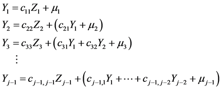
Collecting all the above, we will consider the normal random vector Y, given by (7), where matrix B is any lower triangular matrix and Z is the standard normal j-vector. Write (7) in the form:

(7*)

where m ³ j is the actual dimension of the constructed (final) random vector, say (if m = ¥, one defines, in effect, a stochastic process with time j).

Considering the first –1 lines in (7*) as a system of linear equations, one obtains all as linear combinations of. Substituting these solutions back into (7*) one obtains the following form:

(9)

Realize that transformation (9) is easily reversible.

Assuming that realizations of the random variables are known, we obtain for each:

(10)

where from the above assumed nonsingularity we have c_kk ≠ 0. From (10) it follows that the conditional density of each Y_k, given the values, is normal and for the corresponding conditional expectation we have

while for the (constant) conditional variance we obtain

To adopt the above procedure to our concept of “baseline” T_j versus “in system” Y_j random variables, replace in (9) the independent standard random variables by independent random variables, say, where each T_k has the (“baseline”) normal N(µ_k, s_k) pdf.

Replace transformation (7) by

, (11)

where. Using this change, (10) will be replaced by the following inverse transformation:

(10*)

This yields the conditional pdf of to be the normal

Finally, the general pattern of “creation” of any successive j-variate normal pdf can be explained as follows.

Given are the first j – 1 lines of transformation (11) in the form:

(12)

for some. (Realize that the joint normal pdf of the random vector was defined in j – 1 “previous” steps. In particular for j – 1 = 1, it is the univariate normal N(µ₁, |c₁₁|s₁) density of the variable Y₁.)

We may assume that the next baseline random variable T_j, originally having the N(µ_j, s_j) pdf, is incorporated to the “system” by transforming

This transformation is thought of as adding to (12) the following j-th line:

(13)

[“Physically” this could mean that the variables “become” explanatory (“stresses”) for the “new” variable Y_j obtained from T_j that (originally) was independent from these stresses].

From (13) one can determine the conditional pdf of Y_j, given any realization of the random vector, as the following normal pdf in y_j:

.

Thus, as the j-th “object” (originally independent from the “system” and characterized by the random quantity T_j) was “put into the system” the quantity T_j turns to the quantity Y_j and, in parallel, the parameters µ_j and s_j of its normal density are turned into and, respectively, while normality is preserved.

Clearly, the new value of the (conditional) expectation became the continuous (here linear) function

of realizations while unfortunately the new value of the standard deviation does not depend on but remains constant even if multiplied by the specific, determined by the “system”, number c_jj. This can be “made up” if we allow the number c_jj in (13) to be dependent on, but then the so obtained multivariate FF-normal distribution ceases to be normal since (13) ceases to be linear.

As we have shown also in multivariate cases, the origin of the “parameter dependence method for the construction”, lies in the construction of the multivariate normal distributions. Recall that having defined the conditional pdf and the joint pdf we automatically have the joint pdf as the simple arithmetic product of the two. In the case just considered, all the densities are (arbitrary with the accuracy to the rotations in R^j ) multivariate normal.

Preserving the general spirit of the multivariate normal pdf derivation, let us extend all the Equations (13) for by allowing the translations to be any nonlinear continuous function of and replacing the constant c_j,j by any continuous function of the same variables. Now, for any (13) may be rewritten into the following “triangular” (see Filus, Filus and Arnold [12] ) form:

(13*)

where F_j() and Y_j() are arbitrary continuous functions and.

From (13*) we obtain its inverse:

(13**)

and then for each observation of the conditional pdf of as follows:

(14)

It is clear that the sequence of the densities (14) together with the normal initial density g₁(y₁) of Y₁ uniquely determines the m-variate FF-normal pdf of the random vector. Remarkably, this non-normal density has its natural representation as the product of m normal densities:

(15)

However, the marginal pdfs of are not normal anymore.

The main conclusion which follows the considerations in Sections 6.2 - 6.4 may be stated as: There is a generic relationship that associates the construction method of the parameter dependence with the stochastic dependence structure present within the multivariate normal distribution of any dimension.

As an example of this relationship realize that the transformations (13) and (13*), when applied to the independent normal random variables, define multivariate normal and FF-normal pdfs respectively. They produce other m-variate probability distributions if the normality assumption for T_j is dropped.

Let now be independent random variables all having the standard exponential pdf:

.

Applying to the random vector transformation (13*) and then (13**) for, one obtains the joint density of the resulting random vector to be given by the product of m factors (15), where according to first row of (12) we have and according to (13**)

where the latter is the two parameter exponential density with respect to y_j for.

Another interesting case of the m-variate FF-Weibullian pdf can be obtained by applying transformations (13*) to m independent Weibullian random variables. An even more general class of FF-Weibullians one obtains using the pseudopower transformations (see Filus and Filus [4] ) instead of the pseudoaffine (13*) which actually is a special case of the pseudopower. 

All these distributions (including the m-variate normal) can as well be obtained by direct use of the “parameter dependence pattern” which produces more m-variate models than the considered above transformations. On the other hand existence of the defining transformations facilitates an underlying statistical analysis and simulations.

7. Other Parameter Dependence Paradigms in the Literature

Some paradigms, applied in the reliability literature, are exactly those of the “parameter dependence” that we describe in this paper. However, in most of the cases they are not directly related to the problem of construction of multivariate probability distributions (so, also are different from the “conditioning” procedures in [9] [10] ; see above, Section 5). There are two such subjects that we discuss in the following.

7.1. The Accelerated Life Testing

When testing the life times of some high reliability products, the stresses usually encountered such as temperature, humidity, voltage sometimes are kept on significantly higher than usual levels in order to make the life times shorter than they are in normal conditions. The so obtained data (a “sample”) is then extrapolated into those (hypothetical) life times that would, possibly, be obtained under the regular values of the stresses. Existence of rules, that associate the products’ life times with values of the stresses applied, is necessary for performing proper extrapolations. Several such rules, typically known as the Arrhenius or Eyring (see, Meeker and Escobar [13] , Nelson [14] and [15] an internet source) relationships, are based on physical and chemical considerations on the rates of some chemical reactions that give rise to a given unit’s failure. The obtained models, in general, allow determining the ratio of life times of the same product under higher and under normal temperature or, in the case of the Eyring model, some other physical quantities that play the role of the stresses (see, [13] , formula (18.5) page 476). Methods like that (i.e., the so called SAFT models [13] ) directly relate the (life) times by means of a simple coefficient called the “acceleration factor”.

Unfortunately, with this method the simplicity often comes along with inaccuracy of the predictions. Other methods apply the “Proportional Hazards Relationships” known also as Cox Model (see Cox [16] ) which instead of times relate hazard rates.

More recently ([15] ), the relationships between the life times under different stresses are related indirectly through their probability distributions via distribution’s parameter in that way that considers distribution’s parameter as a function of a given stress (mostly temperature, humidity, pressure, voltage). Those relationships, even if considered in a different context, obey the same paradigm (of the parameter dependence) as that considered in this paper in association with the construction of the multivariate probability distributions.

In what follows we discuss the differences.

1) The generality of the “parameter dependence theory” we built in this paper, is significantly higher than the very special case applied to the accelerated life testing theory. There are three reasons for that. 

Firstly, in our approach the subject of constructing conditional probability distributions is not limited to the life testing, and not even to the “stress-life time” pattern only. The range of applications of our theory is very wide, including many biomedical (see, Collett [17] ) and econometric relationships, (see, Filus and Filus [11] also Filus, Filus and Krysiak [18] ).

Secondly, in the paradigm we consider, the relation between a parameter and stress (or any other random quantity) is given by an arbitrary continuous function, while the number of such functions applied in association with the accelerated life time testing is very limited. Actually, the functions are restricted to few “models” such as the Arrhenius, Eyrie, inverse power law, log-linear, and not many more (see, for example, the Eyring-Weibull model in [15] , Section 5). Those models were obtained from physical and chemical considerations that are only valid for some simple failure (degradation) mechanisms while very often real failure mechanism is too complicated to be analyzed that way.

Our idea is to omit the complicated physical or chemical phenomena that often are poorly understood and to apply two steps purely empirical approach.

Speaking roughly, the first step is an “educated guess” (for choice of a proper function) and the second is statistical verification of this guess.

Thirdly, in our theory we may consider an arbitrary parameter of an arbitrary probability distribution as a stress dependent, while, according to our knowledge (see, for example, [15] ), the only life time distributions so far considered in the accelerated life testing are exponential, Weibullian, and lognormal (normal), and for each the distribution only one parameter is taken under consideration.

2) Besides the generality (of the constructed conditional distributions) our concept also differs with regard to the purpose. Namely, independently of the conditional distributions construction, we also have the construction of bivariate and multivariate probability distributions such as the FF-normal, FF-exponential, FF-Weibullian, FF-gamma and other (for comparison with similar “conditioning methods” of construction present in the literature, see Section 5). 

The construction of high dimension multivariate distributions based on parameter dependence can easily be extended to Markovian and non-Markovian (still simple!) stochastic processes (see Filus and Filus [11] ). The latter constructions seem to be rather unique in the literature.

7.2. Load Control and Load Sharing

1) Other than the accelerated life testing subject, where the “parameter dependence paradigm” is applied, is a set of problems centered around the notion of “load optimization” (see Filus [19] [20] , Levitin and Amari [21] , Nourelfath and Yalaoui [22] and others). This relatively new topic can be described as follows. Some working systems, such as cargo transporting trucks, trains, electric power lines, highways, computer processors, or other systems supporting varying amounts of load, require control of that load. On the one hand more load yields more gain, but, on the other hand, load (as stress) increment yields a corresponding increment of the system’s failure rate which, in turn, depends on certain parameters [20] . The optimization problem can be formulated in several ways ([20] [21] ) but, in all cases, the main idea is to balance between an expected gain that follows a good (load) transportation and the loss in reliability of the transporting medium which decreases the overall gain. Thus, for some (optimal) value of the load to be found, the pure expected gain earned by the system is maximal. In this framework the relationship between stress (the load) and some parameters of the system life time probability distribution (failure rate) is vital for finding a proper model. As examples of such relations, the power and exponential functions of the load were chosen in [20] .

2) Similar application of the parameter dependence pattern also occurs when “load sharing phenomena” takes place. Suppose that we have a parallel system supporting a load such as several engines aircraft or two electric power lines. Failure of any system’s component may cause the total load to be redistributed among fewer components, so that the load on each of them increases by some predictable value. Now we may encounter either the load optimization problem [21] or simply the task of determination of system’s life time probability distribution (see Freund [23] for the exponential case as well as Lu [24] and Filus [25] for Weibullian and lognormal cases). In all these cases the parameter dependence pattern is involved or it is desirable to apply it to get a deeper insight into the underlying stochastic phenomena.

Remark. As a final remark, let me mention the relationship between the parameter dependence presented in this paper, and the stochastic dependence based on models initiated in 1961 by Freund [23] . Besides some similarity the most basic difference lies in the fact that in the Freund scheme the system components act independently until the first failure. In general, the components successive failures cause the total load to be shared by fewer and fewer remaining components, affecting their failure rates (via the parameters).

Quite opposite to that, in the models we introduce, the component interactions take place only when the components work. Any failure of a system component stops its influence on the remaining components’ life times. Therefore, the two paradigms, the “Freund’s load sharing” and our “parameter dependence”, are “disjoint” and in a sense “complementary”. In reality, both (physical) phenomena may take place at the same time and it seems to be quite possible in the future to construct stochastic models (i.e., multivariate probability distributions) that would obey both paradigms.

Nevertheless, we stress the generic relation of all the multivariate probability distributions based on the parameter dependence with the multivariate Gaussians.

References

- Filus, J.K. and Filus, L.Z. (2013) A Method for Multivariate Probability Distributions Construction via Parameter Dependence. Communications in Statistics: Theory and Methods, 42, 716-721. http://dx.doi.org/10.1080/03610926.2012.731549
- Filus, J.K. and Filus, L.Z. (2000) A Class of Generalized Multivariate Normal Densities. Pakistan Journal of Statistics, 16, 11-32.
- Filus, J.K. and Filus, L.Z. (2007) On New Multivariate Probability Distributions and Stochastic Processes with Systems Reliability and Maintenance Applications. Methodology and Computing in Applied Probability, 9, 426-446,
- Filus, J.K. and Filus, L.Z. (2006) On Some New Classes of Multivariate Probability Distributions. Pakistan Journal of Statistics, 1, 21-42.
- Filus, J.K. and Filus, L.Z. (2008) On Multicomponent System Reliability with Microshocks-Microdamages Type of Components’ Interaction. Proceedings of the International Multiconference of Engineers and Computer Scientists, Lecture Notes in Engineering and Computer Science, Hong Kong, 19-21 March 2008, 1945-1951.
- Filus, J.K. and Filus, L.Z. (2010) Weak Stochastic Dependence in Biomedical Applications. American Institute of Physics Conference Proceedings 1281, Numerical Analysis and Applied Mathematics, III, 1873-1876.
- Kotz, S., Balakrishnan, N. and Johnson, N.L. (2000) Continuous Multivariate Distributions (Vol. 1). 2nd Edition, J. Wiley & Sons, Inc, New York, 217-218. http://dx.doi.org/10.1002/0471722065
- Barlow, R.E. and Proschan, F. (1975) Statistical Theory of Reliability and Life Testing. Holt, Rinehart and Winston, New York.
- Arnold, B.C., Castillo, E. and Sarabia, J.M. (1999) Conditional Specification of Statistical Models. Springer Series in Statistics, Springer Verlag, New York.
- Castillo, E. and Galambos, J. (1990) Bivariate Distributions with Weibull Conditionals. Analysis Mathematica, 16, 3-9. http://dx.doi.org/10.1007/BF01906769
- Filus, J.K., Filus, L.Z. (2008) Construction of New Continuous Stochastic Processes. Pakistan Journal of Statistics, 24, 227-251.
- Filus, J.K., Filus, L.Z. and Arnold, B.C. (2010) Families of Multivariate Distributions Involving “Triangular” Transformations. Communications in Statistics—Theory and Methods, 39, 107-116.
- Meeker, W.Q. and Escobar, L.A. (1998) Statistical Methods for Reliability Data. John Wiley & Sons, Inc., New York.
- Nelson, W. (1990) Accelerated Testing: Statistical Models, Test Plans and Data Analysis. Wiley, New York. http://dx.doi.org/10.1002/9780470316795
- (2013) www.ReliaWiki.org/index.php/Accelerated_Life_Testing_Data_Analysis_Reference
- Cox, D.R. (1972) Regression Models and Life Tables (with Discussion). Journal of the Royal Statistical Society, B74, 187-220.
- Collett, D. (2003) Modeling Survival Data in Medical Research. 2nd Edition, Chapman @ Hall/CRS A CRC Press Company, London, New York, Washington, D.C.
- Filus, J.K., Filus, L.Z. and Krysiak, Z. (2013) Analytical Statistical and Simulation Models Utilized in Modeling the Risk in Finance. 5th International Conference on Risk Analysis, Tomar, Portugal, 30th May-1st June.
- Filus, J.K. (1986) A Problem in Reliability Optimization. Journal of the Operational Research Society, 37, 407-412.
- Filus, J.K. (1987) The Load Optimization of a Repairable System with Gamma Distributed Time-to-Failure. Reliability Engineering, 18, 275-284. http://dx.doi.org/10.1016/0143-8174(87)90032-1
- Levitin, G. and Amari, S.V. (2009) Optimal Load Distribution in Series-Parallel Systems. Reliability Engineering and System Safety, 94, 254-260. http://dx.doi.org/10.1016/j.ress.2008.03.001
- Nourelfath, M. and Yalaoui, F. (2012) Integrated Load Distribution and Production Planning in Series-Parallel Multistate Systems. Reliability Engineering and System Safety, 106, 138-145. http://dx.doi.org/10.1016/j.ress.2012.06.006
- Freund, J.E. (1961) A Bivariate Extension of the Exponential Distribution. Journal of the American Statistical Association, 56, 971-977. http://dx.doi.org/10.1080/01621459.1961.10482138
- Lu, J. (1989) Weibull Extensions of the Freund and Marshal-Olkins Bivariate Exponential Models. IEEE Transactions on Reliability, 38, 615-619. http://dx.doi.org/10.1109/24.46492
- Filus, J.K. (1991) On a Type of Dependencies between Weibull Life times of System Components. Reliability Engineering and System Safety, 31s, 267-280. http://dx.doi.org/10.1016/0951-8320(91)90071-E