Applied Mathematics
Vol.3 No.10(2012), Article ID:23380,9 pages DOI:10.4236/am.2012.310170
Simulating Solute Transport in Porous Media Using Model Reduction Techniques
1Civilian Nuclear Programs, Los Alamos National Laboratory, Los Alamos, USA
2Computational Earth Sciences Group, Los Alamos National Laboratory, Los Alamos, USA
3Energy and Infrastructure Analysis, Los Alamos National Laboratory, Los Alamos, USA
Email: robinson@lanl.gov, zhiming@lanl.gov, dmp@lanl.gov
Received August 21, 2012; revised September 21, 2012; accepted September 28, 2012
Keywords: Model Reduction; Solute Transport; Proper Orthogonal Decomposition
ABSTRACT
In this study, we introduce a numerical method to reduce the solute transport equation into a reduced form that can replicate the behavior of the model described by the original equation. The basic idea is to collect an ensemble of data of state variables (say, solute concentration), called snapshots, by running the original model, and then use the proper orthogonal decomposition (POD) techniques (or the Karhunen-Loeve decomposition) to create a set of basis functions that span the snapshot collection. The snapshots can be reconstructed using these basis functions. The solute concentration at any time and location in the domain is expressed as a linear combination of these basis functions, and a Galerkin procedure is applied to the original model to obtain a set of ordinary differential equations for the coefficients in the linear representation. The accuracy and computational efficiency of the reduced model have been demonstrated using several one-dimensional and two-dimensional examples.
1. Introduction
Accurate predictions of radionuclide transport in general come from process models, which are defined as detailed flow and contaminant transport model that best replicate the available data for a site. They usually are the most complex and sophisticated models of flow and transport at a particular site. A significant technical issue arises when one tries to use those model results in probabilistic systems modeling: it is impractical to directly solve the computationally intensive model for each Monte Carlo realization that would be necessary to properly span the range of uncertainty for every model parameter.
On contrast to process models, systems models have been proposed to represent complex process models with simplified models that are suitable for Monte Carlo analysis. Systems models incorporate streamlined versions of one or more process models, along with uncertain estimates of the contaminant source term. Systems models integrate knowledge of all of the processes relevant to assessing risk, and therefore are critical to support remedies or decisions to monitor groundwater. Process models synthesize knowledge of one component of the transport path; the systems models integrate knowledge of all aspects of contaminant transport.
The groundwater pathway in the systems model should be an abstraction model that we believe captures the essential features of the groundwater process model, although there is a risk that the simplification process will filter out something important. When the groundwater pathway is simulated in a process model, it is generally not practical to embed the entire model in the systems model-computational limitations intercede. Consequently, we often settle for one or a few simplified models. These simplified models are called abstraction models. Within these simplified or other types of transport modules, parameters that can be varied in a probabilistic analysis include the groundwater velocity, dispersion coefficient, and sorption parameters. In the best case, the process model is used to justify these parameter distributions, but often this is not done in great detail due to the complexity of the process models and the lack of a convenient tool to formally abstract the process model results. The result may be a systems model that does not fully consider, or indeed even contradicts, one or more of the process models. The credibility of the systems model is placed in jeopardy when this happens.
If an efficient and accurate model abstraction procedure can be implemented for groundwater contaminant transport, we largely avoid the issue of justifying the validity of our abstraction model: the original process model is effectively incorporated in the systems model. Alternatively, if a modeling analysis stops short of systems analysis, the reduced model can still be used to explore uncertainties much more efficiently, thereby allowing better sensitivity analyses to be conducted.
To date, methods for proceeding from complex process models to simplified systems models have not been formally determined or defined. In this study, a method is developed to obtain efficient and accurate reduced models, alternatively referred to as abstraction models. The technique, called the proper orthogonal decomposition (POD), also known as principal component analysis or Karhunen-Loeve expansion, uses the results from a process model as “data” that provides the basis for a reduced model. The procedure, in general terms, calls for the running of the process model, in this case a contaminant transport simulation, forward in time, recording “snapshots” of contaminant concentration. The mathematical technique transforms the results into a set of basis functions that span the behavior of the transport problem throughout the model domain. The reduced model is then constructed by assuming that the solution of the transport problem can be formulated as a linear combination of the basis functions. A Galerkin procedure using the basis functions results in a small set of ordinary differential equations that are solved in time.
There are a variety of applications in various fields of science for which this technique has been applied. For example, researchers in the field of fluid dynamics have used POD methods to discern so-called coherent structures within a turbulent flow field [1], and to characterize the spatio-temporal patterns in two-phase, fluidized bed reactors [2]. Due to the need for compact models suitable for integration into process control systems, the techniques have been applied to the modeling of non-linear heat transfer [3], natural convection [4], and transport of chemicals in chemical vapor deposition (CVD) reactors [5,6]. In the field of groundwater hydrology and reservoir engineering, techniques to develop reduced models have been explored [7-9], although these applications focus on fluid flow rather than contaminant transport.
An excellent summary of the underpinning theoretical development of POD is presented by [10], and several of the aforementioned references contain detailed descriptions of the implementation of the POD technique. Of greatest relevance in the present study are the CVD model studies [5,6]. In these models, fluid flow (a carrier gas) is assumed to be at steady state, and a reacting chemical species is transported in the fluid. Except that the flow is compressible in the CVD case, this is analogous to the problem of chemical transport in groundwater. Thus, although the POD technique has not been developed for contaminant transport in groundwater, the scope of work required to develop this capability is reasonably constrained due to this previous work.
2. Transport Equations
The governing equation for transport of a single solute in porous media can be written as [11]:
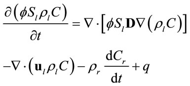 (1)
(1)
subject to an initial condition 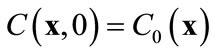 and appropriate boundary conditions. Here f is the porosity, Sl is the liquid saturation, rl is the liquid density, C is the solute concentration, D is the dispersion tensor, ul is the Darcy velocity, Cr represents the adsorption of the solute onto the porous media, rrdCr/dt is an equilibrium sorption term, and q is sources or sinks. All parameters in Equation (1) can be space-dependent, but for simplicity the coordinate
 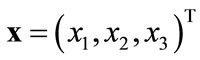 has been suppressed. The general equilibrium model for adsorption of species onto the porous media is given by [12]
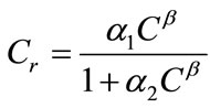 (2)
(2)
where α1, α2, and β are parameters defining different sorption-isotherm models. In this study, the linear isotherm model (α1 = Kd, α2 = 0, and β = 1) is used: Cr = Kd C, where Kd is the partition or distribution coefficient.
If we assume that flow is in saturated porous media at the steady state condition, it follows that rl, D, and ul are independent of time, and saturation Sl = 1. In this case, Equation (1) can be simplified as
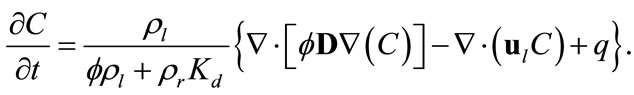 (3)
(3)
This is the full model we deal with in this study. Given appropriate initial and boundary conditions, as well as other parameter fields such as permeability, one can first solve for the velocity field and then the concentration field from Equation (3).
3. Proper Orthogonal Decomposition (POD)
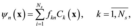
Let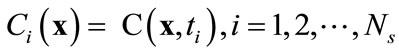 , denote a set of Ns observations (or snapshots) of a state variable (in this case, solute concentration) observed or simulated from the full model run at time ti,
 . The basic idea of the POD method is to find a set of functions
 , called basis functions that have a structure typical of the members of the ensemble
 . The basis functions are chosen to give the best representation of the ensemble of snapshots, which maximizes
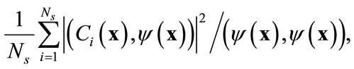 (4)
(4)
where 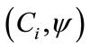 is the inner product of the basis function
  and the concentration field
 . It can be shown that the basis functions can be expressed as a linear combination of snapshots [10]:
 (5)
(5)
where fkn is the kth component of the nth eigenvector of the kernel K that is computed from
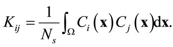 (6)
(6)
By Equation (5), each snapshot can be reconstructed exactly using these basis functions as
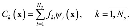 (7)
(7)
To summarize, for a given ensemble of Ns snapshots, one first computes the kernel K from Equation (6) and solves the eigenproblem KF = lF, which gives Ns eigenvalues ln,  , sorted from largest to smallest, and their corresponding eigenvectors
 ,
, . The basis functions are computed from Equation (5) and any snapshot can be reconstructed using Equation (7). Since the matrix K is real, symmetric, and positive semi-definite, all eigenvalues are non-negative. The importance of the nth eigenvectors depends on its relative “energy”, characterized by the ratio of the nth eigenvalue to the sum of all eigenvalues (total energy):
  . In many cases, the first few eigenvalues carry most of the total energy and thus concentration C(x) in Equation (7) can be approximated by truncating the first M terms (
 ).
).
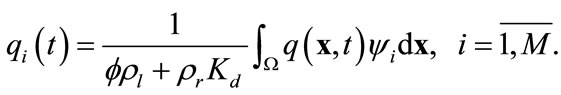
To find the spatial distribution of concentration at a time that is not in the ensemble of snapshots, one has to solve for the coefficients in Equation (7). In the following section, a reduced model is introduced, in which ordinary differential equations for these coefficients are derived from the original (partial differential) transport equations.
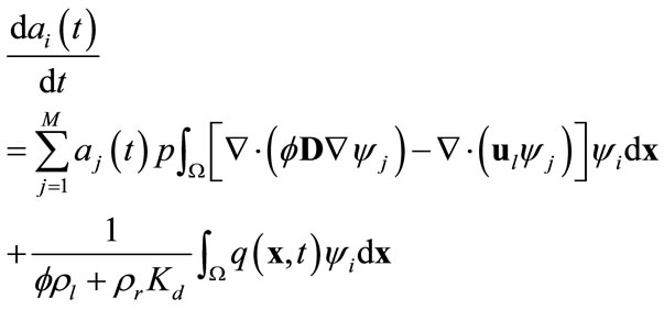
4. Reduced Model
Suppose that the full model, i.e., Equation (3), is solved to obtain a set of snapshots of the concentration distribution C(x, ti), . Based on the algorithm described in the previous section, one can find a set of basis functions
  Then the Galerkin’s method can be employed by seeking an approximation of concentration C(x, t) as
 (8)
(8)
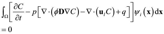
where M < Ns, and am are time-varying coefficients that are independent of spatial locations. The physical mean of (8) is that the concentration field is approximated by a linear combination of some pre-determined, space-dependent “structures”, weighted by some time-dependent coefficients. Since  in (8) is an approximation of the true concentration, replacing
  in the full model, i.e., (3), by
  will produce a model error. In the Galerkin’s method, this error is forced to be orthogonal to all basis functions, i.e.,
 (9)
(9)
for , where
 . Here the orthogonality of any two functions is defined as the integration of the product of two functions over the simulation domain being zero. Substituting (8) into (9) and recalling the orthogonality of basis functions yield
 (10)
(10)
which can be written as
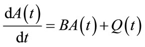 (11)
(11)
where ,
,  and
and
 are defined as
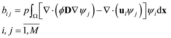 (12)
(12)
and
 (13)
(13)
The initial condition for Equation (11) is derived from the original initial condition C(x, t) = C0(x):
 (14)
(14)
Thus the partial differential equation (PDE) has been reduced to a system of M ordinary differential equations (ODE). Provided that M is fairly small, the reduction in computational time should be significant compared to the numerical solutions of the PDE in the original model.
5. Illustrative Examples
In this section, several examples are presented to illustrate how the model reduction techniques can significantly reduce computational efforts in solute transport in porous media, while retaining accuracy. This is accomplished by comparing results from the reduced models against those from the full model runs. Note that, in solving the full model numerically, it is quite often that numerical errors may be introduced. To avoid this, in the first two examples, simple one-dimensional transport problems were chosen because analytical solutions for these simple cases are available, which made it easy to assess the accuracy of the reduced model.
5.1. One-Dimensional Solute Transport with Linear Sorption
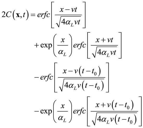
In the first example, we consider a one-dimensional transport problem in a saturated column of 1 m in length, uniformly discretized into 200 elements. The hydraulic conductivity is a constant Ks = 1.0 m/day for the entire column, and the flow is driven by a hydraulic gradient of J = 0.001, which produces a uniform flow with Darcy velocity of 1.1813 × 10⁻⁸ m/s. Other transport parameters are given as: the dispersivity coefficient αL = 0.03333 m, partition coefficient Kd = 0.1, water density rl = 1000.0 kg/m3, rock density rr = 2500 kg/m3, and porosity f = 0.25. Under the given initial condition C(x, 0) = 0, a fixed concentration C(x, t) = 1.0 at the inlet (x = 0), and a zero concentration gradient ¶C(x, t)/¶x = 0 at x = ¥, this problem can be solved analytically [13]:
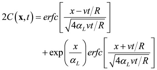 (15)
(15)
where 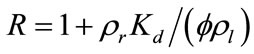 is the retardation factor, and erfc is the complementary error function. Twenty-five concentration snapshots are computed using Equation (15) at time t = nDt, where Dt = 20 days and n ranges from 1 to 25. Some selected snapshots are illustrated in Figure 1.
Using these 25 snapshots, the kernel K is computed from (6), and the eigenvalues and eigenvectors associated with this kernel are solved from KF = lF. These eigenvalues and eigenvectors depend significantly on the choice of snapshots. It is critical that each snapshot be significantly different from all others.
The eigenvalues for this set of snapshots are depicted in Figure 2. The figure indicates that the first eigenvalue carries about 91% of the total energy and the first 6 eigenvalues carry more than 99.99% of the total energy. The ratio of the accumulative energy to the total energy is a measure that can be used to determine the number of modes needed to achieve a given accuracy.
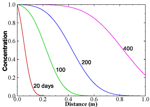
Figure 1. Selected snapshots computed from Equation (15) for the one-dimensional solute transport with linear sorption.
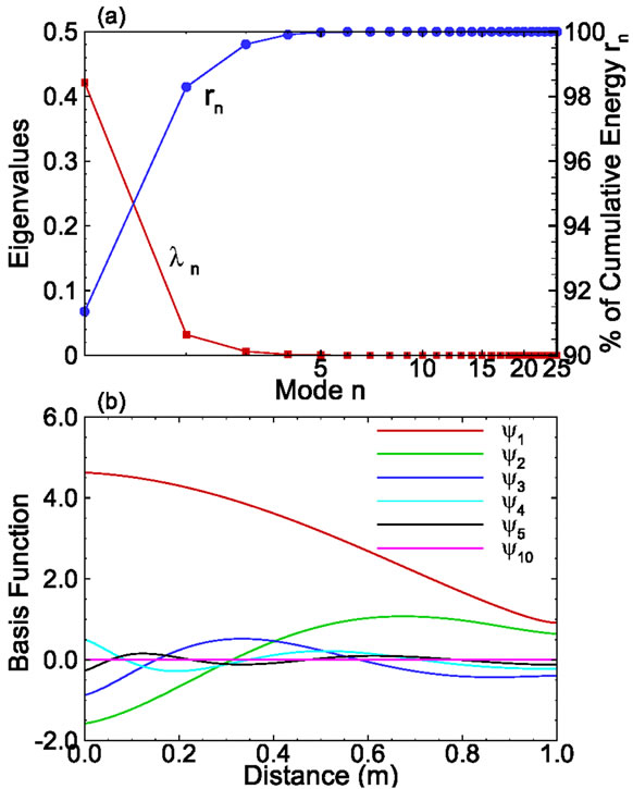
Figure 2. (a) The eigenvalues and their cumulative value as functions of modes; and (b) Selected basis functions for onedimensional solute transport with linear sorption.
The first few basis functions are illustrated in Figure 2(b). It is seen from the figure that the magnitude of the first basis function is much larger than that of other basis functions. In addition, the magnitude decreases as the mode number increases, which makes it possible to approximate the concentration field using only a few terms rather than Ns (=25) terms.
Based on these basis functions, all snapshots can be reconstructed using Equation (7). Comparisons of the true snapshots and reconstructed snapshots indicate that at most 6 basis functions are enough to reconstruct these snapshots with sufficient accuracy. Of course, in general, the number of basis functions required to obtain an accurate solution will depend on the parameters (Ks, and αL, L) in the solute transport problem.
The spatial distribution of solute concentration at any given time can be derived from solving the reduced model. The ordinary differential Equation (11) with the initial condition (14) was solved using the fourth-order Runge-Kutta method with a time step of Dt = 1000 s. In particular, the ensemble of those snapshots can be solved from the reduced model (rather than reconstructed from (7). Four selected concentration distributions computed from the reduced model, as functions of the number of basis functions included, are illustrated in Figure 3. Also plotted in the figure is the true (exact) solution from Equation (15). The figure clearly shows that the accuracy of the estimated concentration distribution depends on the number of basis functions included. For this example, including 10 basis functions is enough to produce very accurate results as compared to the exact solutions.
It should be pointed out that, if the number of basis functions included in the reduced model is not enough, the results could be completely wrong. As illustrated in Figure 3, for snapshots 10 and 20, when a small number of basis functions were used, the concentration value is larger than 1.0, which is physically impossible, as the concentration at the inlet is 1.0.
It is interesting to investigate how well the reduced model can predict the concentration distribution at an elapsed time that is different from those times at which the ensemble of snapshots are taken. Figure 4 compares the concentration profiles at time t = 75 and 525 days computed from the analytical solution and those solved from the reduced model with 15 basis functions. Note that t = 525 days is larger than the maximum time of all snapshots used in constructing the reduced model. The comparison in the figure demonstrates that the reduced model can reproduce the true solution accurately.
5.2. One-Dimensional Transport with Pulse Input
In the second example, all transport parameters are the same as in the previous example except that (1) the partition coefficient Kd is zero in this case, and (2) instead of a fixed constant concentration at the inlet (x = 0), a unit pulse input is imposed at the inlet for a duration of 5 days. For this simple case, analytical solution is also available [13]:
 (16)
(16)
where t0 is the duration of the pulse input, which starts at zero. Using this equation, 25 snapshots were calculated from t = 10 to 250 days at an increment of 10 days. Several selected snapshots are illustrated in Figure 5.
Following the POD method, the kernel K was computed from these 25 snapshots using (6); eigenvalues and eigenvectors were solved from KF = lF; and then basis
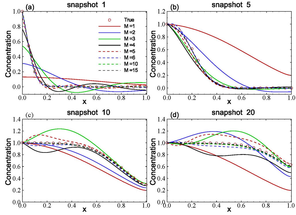
Figure 3. Accuracy of computed snapshots using the model reduction method with different numbers of basis functions.
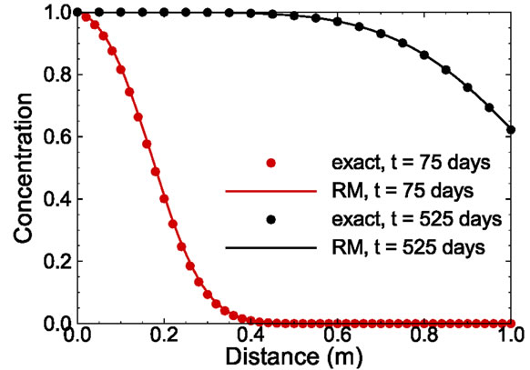
Figure 4. Comparison of exact solution and reduced model solution at time t = 75 days and 525 days.
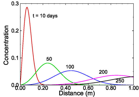
Figure 5. Selected snapshots computed from Equation (16) for the one-dimensional solute transport with pulse input.
functions were computed using (5). The set of eigenvalues as a function of the mode is depicted in Figure 6(a). Unlike in the previous case where the first eigenvalue carries about 90% of energy, in this case the first one has only 40% of energy and the first 8 eigenvalues carry about 99.99% energy, which means that more basis functions may be required to approximate the solution. This can also be seen from Figure 6(b), where the relative magnitudes of the first few basis functions are more or less the same, while in the previous example the magnitude of the first basis function is much larger than that of other basis functions. A larger number of required basis functions may be attributed to the fact that the patterns of different snapshots are quite different in this example while in the previous example all snapshots have a very similar pattern.
Figure 7 compares four snapshots computed from the analytical solution and those solved from the reduced model with different numbers of basis functions included in the reduced model. It is seen from the figure that the reduced model with 10 basis functions is accurate enough. We also compared concentration profiles at time t = 75 and 275 days derived from the analytical solution and those from solving the reduced model with 10 basis functions (not shown). Again, the solutions from the reduced model are nearly identical to the true solutions.
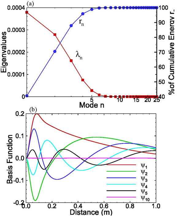
Figure 6. (a) The eigenvalues and their cumulative value as functions of modes; (b) Selected basis functions for the onedimensional solute transport with pulse input.
5.3. Two-Dimensional Solute Transport with Heterogeneous Conductivity and Sorption Coefficients
In the third example, solute transport is modeled in a two-dimensional rectangular domain of size 1 m × 0.5 m, uniformly discretized into 100 × 50 square elements. Nonflow conditions are prescribed at two lateral boundaries. The hydraulic head is fixed at the left and right boundaries as 10.001 m and 10.0 m, respectively, with a hydraulic gradient J = 0.001. The porous medium is heterogeneous in both the hydraulic conductivity Ks and the sorption coefficient Kd. It is assumed that the log hydraulic conductivity Y = ln(Ks) has a normal distribution and is second-order stationary following an isotropic, exponential covariance function with a correlation length of 0.3m. The statistics of the log hydraulic conductivity are given as  = 0 (i.e., the geometric mean of the saturated hydraulic conductivity KG = 1.0 m/day) and
  = 0.693 (the coefficient of variation CV = 100%). Figure 8(a) shows the log hydraulic conductivity field generated using the sgsim code in GSLIB [14]. In this case, the velocity field is no longer uniform in the flow domain and has to be solved numerically. The steady-state, saturated flow problem was solved using the Finite-Element Heatand Mass-Transfer code (FEHM) developed by Zyvoloski et al. [11]. This velocity field was used as input to the solute transport model.
For the transport problem, it is assumed that the initial concentration is zero in the domain and concentration of C(x, t) = 1.0 is fixed at the middle of the upstream boundary, (0.0 m, 0.25 m). It is also assumed the log partition
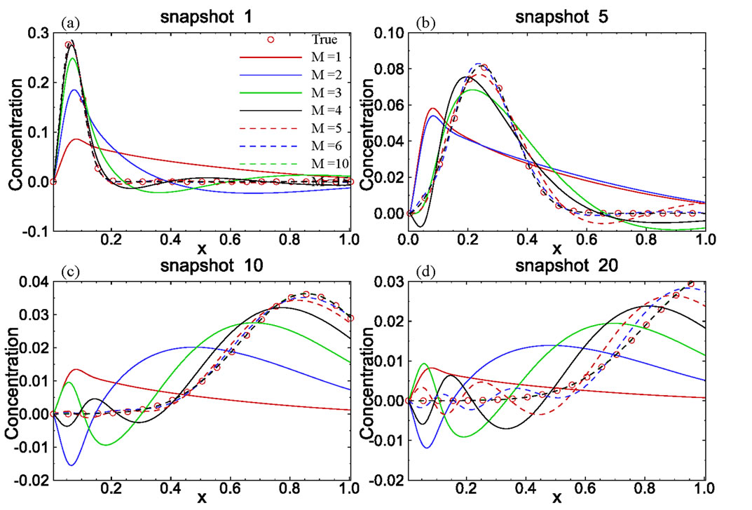
Figure 7. Accuracy of computed snapshots with different numbers of basis functions using the model reduction method for the one-dimensional solute transport with pulse input.
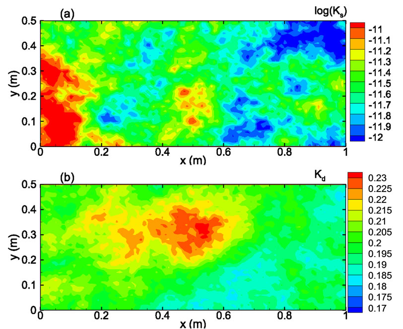
Figure 8. Gaussian random fields for (a) log Ks, and (b) Kd.
coefficient is uncorrelated with the log hydraulic conductivity and that ln(Kd) is also second-order stationary field following an isotropic, exponential covariance function with a correlation length of 0.3 m. The statistics of ln(Kd) are given as  = -1.6094 (i.e., the geometric mean
  =0.2) and
  = 9.95 × 10⁻³ (the coefficient of variation CV = 10%). The spatial distribution of Kd generated using the sgsim code of GSLIB is illustrated in Figure 8(b). Other transport parameters include the longitudinal dispersivity coefficient αL = 0.02 m, and the transverse dispersivity coefficient αT = 10-4 m.
The full transport model was run for 200 days using the FEHM code and the concentration distribution was recorded at t = 10n days, where n ranges from 1 to 20, and these 20 concentration fields were taken as snapshots for the model reduction method. Basis functions were then computed from these snapshots using the POD method, and Equation (11) with initial condition (14) were solved numerically.
Figure 9 compares the spatial distribution of concentration as contour maps at two elapsed times, t = 100 days and t = 200 days, derived from both the full model run and the reduced model with 5 basis functions. The comparison clearly shows that the results from the re-
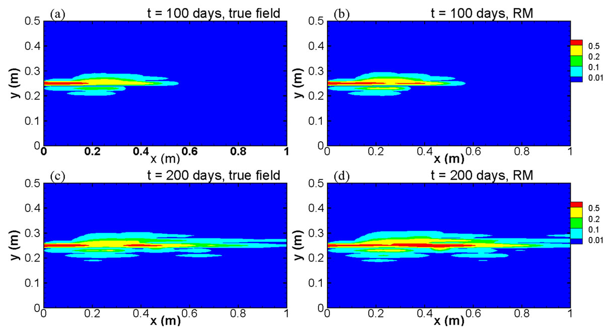
Figure 9. Comparison of true concentration fields and modeled fields using the reduced model at two elapsed times for the case with heterogeneities in both the permeability and the distribution coefficient.
duced model can reproduce the full model results very well, even for a contour level as low as C = 0.01.
To compare the computational efficiency of these two methods, the CPU time required for the full model run was recorded, in which the maximum time step was set to 2 days while the actual size of the time step was automatically adjusted during the solution process by the program itself. For the transport problem as described above, the FEHM code takes 23.3 hours. The computation time needed for the reduced model depends on the time step used in the fourth-order Runge-Kutta method, which is fixed at Dt = 1000 seconds in this case. The CPU time for the reduced model run is only 78 seconds. Of course, this run time will increase if a smaller time step was used or a great number of snapshots and functions is required. However, the comparison of model results from the full model and the reduced model indicates that the time step of Dt = 1000 seconds used in the reduced model is small enough for this problem, and the overall comparison indicates that the number of snapshots and basis functions were sufficient.
6. Conclusions
In this study, we have demonstrated that the advectiondispersion equation can be cast in a reduced model form, and a reduced numerical model can be developed that replicates the behavior of the original model. We have derived, from the original model equations, a method for reducing the transport model, a partial differential equation with unknowns at each numerical grid point, to a small number of ordinary differential equations solved in time. The method consists of running the original model to obtain the snapshots of concentration in the model domain, computing the basis functions for the model using the POD technique, and using these basis functions in a Galerkin procedure to obtain the ordinary differential equations of the reduced model.
The accuracy and computational efficiency of the reduced model have been investigated using several onedimensional and two-dimensional examples with variable conductivity field Ks and sorption coefficient Kd. These examples demonstrate that the reduced model can reproduce the full model results very accurately while the computational time (in terms of the CPU time) required for the reduced model is much less than that required for the full model.
REFERENCES
- G. Berkooz, P. Holmes and J. L. Lumley, “The Proper Orthogonal Decomposition in the Analysis of Turbulent Flows,” Annual Review of Fluid Mechanics, Vol. 25, No. 1, 1993, pp. 539-575. doi:10.1146/annurev.fl.25.010193.002543
- P. G. Cizmas, A. Palacios, T. O. O-Brien and M. Syamlal, “Proper-Orthogonal Decomposition of Spatio-Temporal Patterns in Fluidized Beds,” Chemical Engineering Science, Vol. 58, No. 19, 2003, pp. 4417-4427. doi:10.1016/S0009-2509(03)00323-3
- H. M. Park and D. H. Cho, “The Use of the KarhunenLoeve Decomposition for the Modeling of Distributed Parameter Systems,” Chemical Engineering Science, Vol. 51, No. 1, 1996, pp. 81-98. doi:10.1016/0009-2509(95)00230-8
- H. V. Ly and H. T. Tran, “Modeling and Control of Physical Processes Using Proper Orthogonal Decomposition,” Report CRSC-TR98-37, Center for Research in Scientific Computation, North Carolina State University, Raleigh, 1999.
- A. J. Newman, “Model Reduction via the KarhunenLoeve Expansion Part II: Some Elementary Examples,” Tech. Report T.R. 96-33, Inst. Systems Research, 1996.
- H. V. Ly and H. T. Tran, “Proper Orthogonal Decomposition for Flow Calculations and Optimal Control in a Horizontal CVD Reactor,” Report CRSC-TR98-13, Center for Research in Scientific Computation, North Carolina State University, Raleigh, 1998.
- R. Markovinovic, E. L. Geurtsen, T. Heijin and J. D. Jansen, “Generation of Low-Order Reservoir Models Using POD, Empirical Gramians, and Subspace Identification,” 8th European Conference on the Mathematics of Oil Recovery, Freiberg, 3-6 September 2002.
- T. Heijin, R. Markovinovic and J. D. Jansen, “Generation of Low-Order Reservoir Models Using System-Theoretical Concepts,” SPE Paper 79674, SPE Reservoir Symposium, Houston, 2003.
- P. T. M. Vermeulen, A. W. Heemink and C. B. M. Te Stroet, “Reduced Models for Linear Groundwater Flow Models Using Empirical Orthogonal Functions,” Advances in Water Resources, Vol. 27, No. 1, 2004, pp. 57- 69. doi:10.1016/j.advwatres.2003.09.008
- A. J. Newman, “Model Reduction via the KarhunenLoeve Expansion Part I: An Exposition,” Tech. Report T.R. 96-32, Inst. Systems Research, 1996.
- G. A. Zyvoloski, B. A. Robinson, Z. V. Dash and L. L. Trease, “Summary of the Models and Methods for the FEHM Application—A Finite-Element Heatand MassTransfer Code,” Los Alamos National Laboratory Report LA-13307-MS, Los Alamos, 1997.
- W. L. Polzer, M. G. Rao, H. R. Fuentes and R. J. Beckman, “Thermodynamically Derived Relationships between the Modified Langmuir Isotherm and Experimental Parameters,” Environmental Science & Technology, Vol. 26, 1992, pp. 1780-1786. doi:10.1021/es00033a011
- V. Batu, “Applied Flow and Solute Transport Modeling in Aquifers: Fundamental Principles and Analytical and Numerical Methods,” CRC Press, London, 2006.
- C. V. Deutsch and A. G. Journel, “GSLIB: Geostatistical Software Library,” Oxford University Press, New York, 1992.