ABSTRACT

This article identifies cycles of Gabon GDP, those of its main components (consumption, investment, government spending, exports and imports), and their characteristics (duration, severity and depth), using a band-pass filter and according to the algorithm of Bry and Boschan. Synchronization and the concordance of the cycles of GDP and those of its components are highlighted. Similarly, the contributions of cycles of variables that make up the GDP to the cycles of this greatness are studied according to Stock and Watson’s way (1998).

1. Introduction

After being considered as outdated subject a few decades ago, the study of the business cycle is experiencing a resurgence of interest in favor of international financial crises and sovereign debts within the European Union.

Introduced by [1] of the National Bureau of Economic Research (NBER) business cycle, called a “classic” cycle or cycle of the GDP, according to the authors, composed “of expansions occurring at about the same time in many economic sectors, followed by recessions, constraints and revivals which then fuse to the phase of expansion of the next cycle” (e.g., see [1]).

Traditionally, two types of approaches are being considered to explain the phenomenon of economic cycle in a country: exogenous approaches and endogenous theories. According to the supporters of the trend of exogenous theories, fluctuations are caused by natural phenomena such as sunspots, on the one hand, human phenomena such as population and the clusters of technological progress, on the other hand. For the supporters of endogenous theories, the appearance of economic cycles in a country is linked to the economic activity for itself. Specifically, these theories focus on various factors such as the use of income, the structure of production or over-investment theory, financial variables.

The latest developments of the theory of economic fluctuations concern the Theory of Real Cycles (TRC) and the New Keynesian Economics (NKE). The theory of real cycles is based on pre-Keynesian analyses of Hayek that stress the dynamics of the spread in time and in all the sectors of the shocks. In this regard, it underlines the importance of technology shocks in the explanation of the fluctuations of the activity and the behavior of intertemporal optimization of the type agent in response to the changes occurred in its environment. Thus, the Theory of Real Cycles (TRC) is a theory of cycles at equilibrium. On the contrary, the theory of fluctuations according to the New Keynesian Economics (NKE) endeavours to explain the variations of the economic activity by the slow of the adjustments of prices and wages, the coordination failures, the spreading out of the fixing of prices and wages.

On the empirical level, since the seminal works of [1], the study of cycles resulted in an extensive literature. Among the relatively recent works, we will notably evoke [2].

If the interest taken on the study of cycles in developed countries is old and the literature related to it abundant, it is not so in developing countries where empirical studies are rather, except [3,4] works. Two arguments are generally advanced to justify the relative attractiveness of the study of the economic cycle in developing countries: the absence of appropriate statistical information both at the quantitative and qualitative levels, on the one hand, the fact that developing countries tend to be prone to sudden crises and marked gyrations of macroeconomic variables, which often make it difficult to discern any type of cycle or economic regularities, on the other hand.

Especially in Central Africa, the issue of cycles has not attracted much interest. It is particularly the case of Gabon, a small country open to the outside, with an economy dependent on oil. However, the study of cycles in that country is interesting in that it provides a valuable tool for the implementation of appropriate economic policies.

Leaning on the case of Gabon, the present study is organized as follows: Section 2 identifies cycles of GDP and its components. Section 3 studies the co-movements and the degree of concordance between the cycles of GDP and those of its components. Section 4 analyzes the cyclical contributions of components of GDP. Finally, Section 5 concludes.

2. Identification of the GDP Cycles and Its Components

Like [5], we use the method of band-pass filter of [6] to extract the cycles of Gabon GDP and those of its components. The choice of this method is explained by its ability to provide ample cycles, persistent and to estimate a stochastic tendency.

Indeed, the filter of the passing band of [6] is an extension of the original filter of [7]. The latter decomposes a process balanced of sinusoidal functions, in which is a frequency whose weight is deduced from Fourier’s transformed of the autocorrelogram of the process. This one corresponds to the value of the spectral density of for the frequency.

The method relies on the a priori choice of frequencies defining the cycle. According to Baxter and King, the cycle of temporal series is generally admitted a period comprised between 6 and 32 quarters. The tendency which translates the evolutions of long term or low frequency, admits a period superior to 32 quarters. The irregular, which corresponds to evolutions of very shortterm or high-frequency, admits a period inferior to 6 quarters. So, the extraction of the cycle consists in applying to the process the band-pass filter which keeps those frequencies and cancels the others. So, the cycle is obtained as the difference of the two band-pass filters. The ideal band-pass filter, associated with the frequency w₀, must have a function of transfer of the shape:

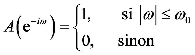(1)

Transformation in Fourier series of is written:

(2)

where;;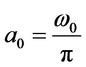 and.

The series issued from the band-pass filter is supplied by the infinite mobile average.

(3)

In practice, the interval of time frequencies is specified by the user according to his intuition on the periodicity of the cycle studied. The contribution of [6] has consisted in proposing a band-pass filter specific to short frequencies which characterize the stationary stochastic processes.

Regarding the dating of cycles, two main methods are commonly used: the nonparametric method of [8] and Markovian models with regime change. In the framework of this study, following [9], we retain the first method. Indeed, Markovian models with regime change face the problem of the robustness of estimates related to the degree of reliability and data quality in developing countries. Moreover, they present imperfections concerning the rule of identification of the points of reversal of cycles [10].

However, the algorithm of [8], which is used by the National Bureau of Economic Research, allows the identification of reversal points (peaks and troughs) of a cycle by a method proposed by [1]. It is summarized in three main steps:

1) The determination of the points of reversal candidate of an annual series retains the following rule:

- y_t admits one trough at t if :

- y_t admits one trough at t if :.

2) The disqualification of reversal points located more or less six months from the beginning or the end of the series.

3) The verification of a perfect rule of alternation between peaks and troughs so that in the presence of a double trough, the smallest value is chosen. In the presence of a double peak, the highest value is retained.

Once dated, the cyclical component can be characterized from the calculation of the following main indicators:

- The depth corresponds to the amplitude of recession or expansion, and it is defined by:

(4)

where x_p is the value of the series with the peak and x_c is the value with the trough of cyclical component.

- The severity summarizes the piece of information contained in the duration and depth. Furthermore, it measures the loss (respectively the gain) achieved by a variable during a contraction phase (respectively an expansion phase). It is calculated using the formula:

(5)

The application of the preceding methods is performed on the data of the Gabonese economy: Gross Domestic Product (GDP) and its components, namely, consumption, investment, government spending, exports and imports. The data are from the World Development Indicators of the World Bank. All the series have been previously transformed into logarithms.

Following [4], the regular changes of the main macroeconomic indicators of developing countries and their frequent exposure to economic crises lead to retain the values 2 and 8 years as the boundaries of the interval of reproduction of cyclical components of the activity and variables of Gabon GDP. According to [11], these values are commonly used by literature to estimate the business cycle. They correspond to the interval of the time frequencies of Christiano and Fitzgerald’s filter. From then on, lower frequencies to correspond to the long term, and those superior to correspond to the short term.

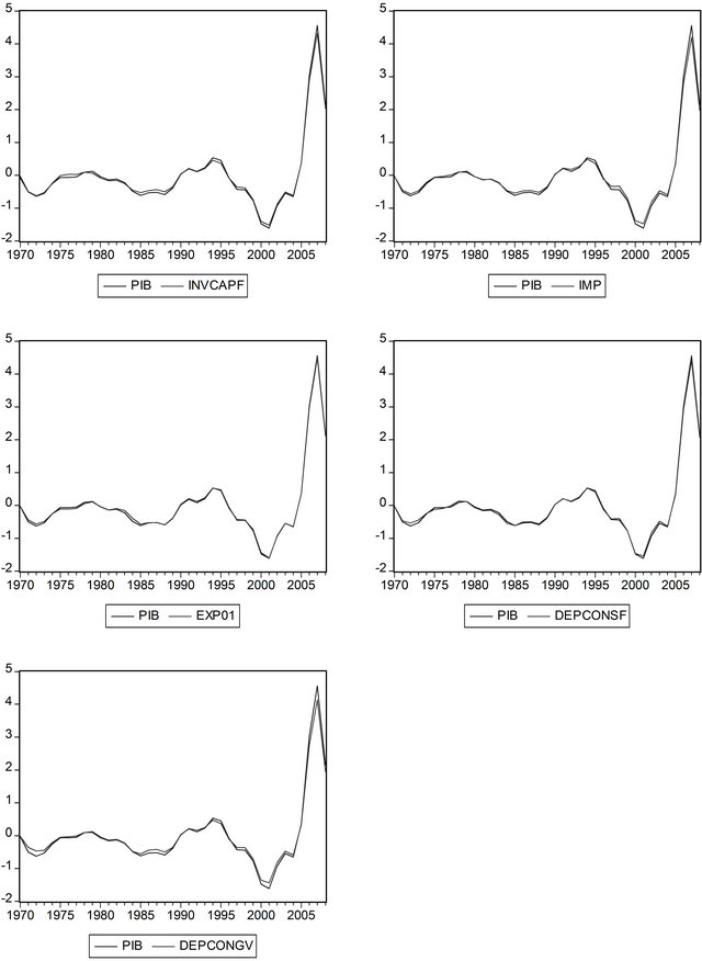
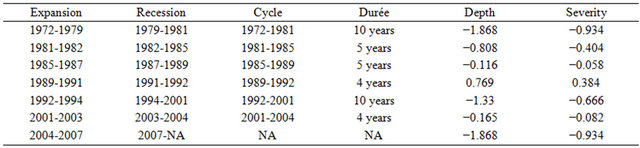
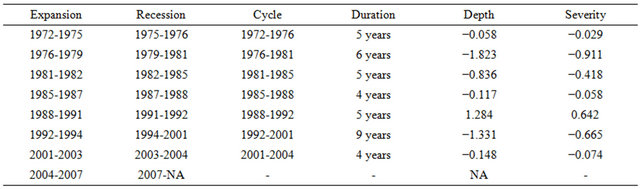
Appendix 1 represents graphs of the GDP components, and Appendix 2 shows tables of their properties. Therefore, we retains the following lessons: For the period going from 1972 to 2007, the empirical analysis highlights six cycles (1972-1981, 1981-1985, 1985-1989, 1989-1992, 1992-2000, 2001-2004) for the GDP of Gabon. With the exception of the cycle of the periods 1972-1981 and 1992-2001 which have a duration of 10 years, the other cyclical periods have a duration comprised between 4 and 5 years.

Over the period 1972-1981, the cyclical evolution of the GDP Gabon shows an expansion phase which runs from 1972 to 1979 and a recession phase between 1979 and 1981. The expansion phase seems to be explained by the favorable impact of the oil shock of 1973, given the overwhelming importance of oil in the Gabonese economy. The severe recession observed, with a shift, over the period 1979-1981 is imputable to the payments crisis Gabon is facing following the proactive fiscal policy conducted in the framework of the achievement of the proceedings of the Conference of Heads of State of the Organization of African Unity (OAU) in 1977 in the country.

Despite the growth recorded over the period 1981-1982, due to the second oil shock, the cyclical evolution of the Gabonese economy is marked by a relative recession until 1985, due to the stabilization of oil prices on the one hand, the effects of the interim plan implemented by the Government as a result of payments crisis, on the other.

Given the shifted effects of the counter oil shock (drastic drop in the price of the barrel of oil) and the depreciation of the U.S. dollar on foreign exchange markets, the cyclical evolution of the Gabonese economy is marked by a sharp recession that culminates in 1987. Taking advantage of the discovery of a new oil field at Rabi-Kounga (off Port-Gentil, the economic capital of Gabon), Gabon economy witnesses another improvement that the growth of the period 1989-1991 translates.

After the 1991-1992 recession, the Gabonese economy has entered a cycle of ten years (1992-2001) successively marked by an expansion phase during the period 1992- 1994, then a recession phase (1994-2001) with a depth (amplitude) and a severity relatively high. The expansion phase seems to be explained by the increase of oil production, due to the exploitation of the Rabi oilfield. However, the recession phase is linked to the economic crisis following the devaluation of the CFA franc.

Finally, the cycle of the GDP of Gabon presents two phases of expansion over the periods 2001-2003 and 2004-2007, due to the rise of the barrel of oil. With respect to fluctuations of the GDP components, the empirical analysis suggests the following observations:

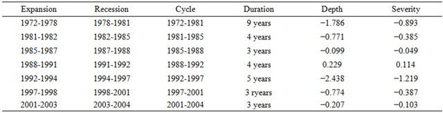
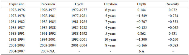
1) The evolution of consumption reveals seven cycles, or no more than that of the GDP. With the exception of the first cycle (1972-1981) which has a term of nine years, the remaining cycles have a duration varying between four and six years. Thus, it appears that the cycles of consumption have a relatively shorter duration than those of GDP. In this respect, one can observe, for example, that the cycle of GDP starting in 1992, ends in 2001, which is a period of ten years. On the other hand, the corresponding cycle of consumption ranges from 1992 to 1997, five years. Precisely on the latter, the recession phase, which marks the end of the cycle (1994-1997), is followed by a new cycle (1997-2001) which highlights the phases of expansion and recession, respectively on the periods 1997-1998 and 1998-2001. Thus, while GDP growth is marked by a recession over the period 1994-2001, that of the final consumption records successively a recession (1994-1997), then during the next cycle, an expansion (1997-1998) and a recession (1998-2001). It therefore appears that the decline of the GDP does not immediately entail the fall in consumption. Indeed, that one comes four years after the starting of recession, what suggests that Gabonese households have a behavior of consumption that translates the taking into account of the phenomena of memory;

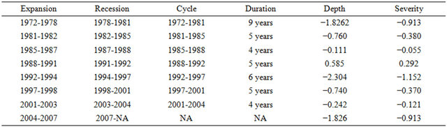
2) The behavior of investment highlights seven cycles, generally having a relatively shorter duration than the cycles of GDP, except for the cycle of the period 1992- 2001 cycle which spans over ten years. That leads to think that, like for consumption, the investment behavior responds with a shift to the cyclical evolutions of the GDP;

3) Similarly, the behavior of the expense of the Government reveals seven cycles which seem to translate the dependence of the fiscal policy of Gabon to the oil conjuncture;

4) The evolution of exports of Gabon also reveals seven cycles, strongly influenced by fluctuations of the price of a barrel of oil, which surprises a little since oil exports of oil account for about 60% to 80% of exports of the country;

5) The empirical analysis highlights seven cycles for imports. These cycles appear to be related to the oil conjuncture. This is understandable since it influences the evolution of terms of trade which are one of the determinants of imports to developing countries.

After making the identification of GDP cycles and those of its components, it seems appropriate, now, to approach the study of co-movements and the degree of concordance.

3. Co-Movements and Concordance Index

The analysis of the co-movements of the phases of expansion and the recession of the cyclic constituents of the activity and those of the variables of the GDP rests on the calculation of crossed dynamic correlations between the stationary cyclic components of one variable of the GDP and those delayed or advanced of the activity y_t–k (k = 0, ± 1, ± 2, ± 3) and on an approximation of the distance-type of the sample by. The step retains the following criterion:

- the constituent is procyclic, ifone has:;

- the constituent is acyclic if;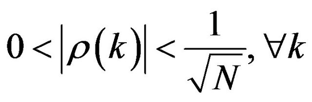

- the constituent is contracyclic if

.

Similarly, the preceding relations can be classified according to the level of significance. Thus, the relationship between the cycles of GDP and those of its components is:

- significative at the threshold 5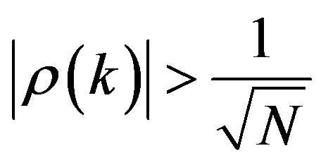% if or if

- significative at the threshold 10% if

Meanwhile, the analysis of the degree of concordance between the cyclical components consists in the construction of the concordance index proposed by [9], which permits to assess the link between the periods of recession and expansion of two series and. Formally, the concordance index between and is calculated as follows:

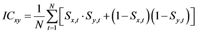(6)

where, for a series considered.

So, when IC_xy = 1, the series and are perfectly in phase. In other words, their phases of expansion and contraction are perfectly juxtaposed. When IC_xy = 0, the and are always in opposite phases, and there is perfect anti-concordance between the two series.

In general, the properties of the concordance index are unknown. So, concerning its degree of significance [9], show that it corresponds to the degree of significance of the coefficient ρ in the estimating of the following linear model:

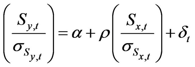(7)

with: a white noise process.

Under the null hypothesis, the serial correlation of errors is harmful to the robustness of the estimation of the model (7). In this case, propose to use the method of the least squares augmented by a HAC procedure to assess the significance of the concordance index from student’s statistics [12].

Empirically, like [13], we study the results of dynamic correlations and indices of concordance in order to determine the co-movements and the degree of concordance between the phases of expansion and recession of different cycles.

The results of the analysis of dynamic correlations are summarized in Table 1 in Appendix 3.

From Table 1 (Appendix 3), it results that the cyclical components of GDP and those of the variables which compose it are contemporaneous, since the maximum value of the correlation coefficient between the cycle of GDP and that of each of the components is obtained when. In other words, there is no shift between the evolution of cycles of the GDP and those of its components. We therefore say that the variables that make up GDP are all procyclical. Moreover, the correlation value of the column shows that in almost 98% of the time, the phases of recession and expansion of the two cycles coincide. Finally, according to the criterion of significance of correlation coefficients, all the coefficients of column are significant since they belong to the interval (0.32-1). The procyclicality of the variables of the GDP is therefore confirmed by the values of correlation coefficients. The positive sign of these coefficients for indicates a positive correlation between the two cycles.

Table 1 (Appendix 3) also shows that the correlation coefficients are relatively high and significant at the threshold 5% for all variables, where. This result suggests the existence of procyclicality of the variables composing the GDP in relation to the latter, with a shift of one period. However, the use of annual data does not permit to accurately determine the duration of this shift. However, the availability of quarterly or monthly data may overcome this constraint.

The calculation results of concordance indices are presented in Table 2 in Appendix 3;

According to the criterion of [9], all concordance indices are significant at the threshold of 5% since the coefficients estimated from Equation (7) are near 0.999, with a probability equal to 0.000 and a coefficient of determination R² which rises at 0.999.

In addition, the table of concordance indices confirms the result of the analysis of cross correlations and suggests a synchronization of the cycles of the variables of GDP with those of that magnitude. Indeed, the relatively high values of these indices (close to 0.5) lead to sustain that all the variables of the GDP are procyclical. Moreover, we note that the values of the concordance index for exports, investment and government expenditure (0.487) are relatively higher than those of the other components of the GDP. What seems to indicate the procyclical character which more marked of these variables in comparison with the GDP.

After analyzing the co-movements and the degree of concordance, let us now see the cyclical contributions of the components of the GDP.

4. The Cyclical Contributions of the GDP Components

The analysis of the contributions of the cycles of the components of the GDP to the cycles of this variable is made according to a method proposed by [13]. It is based on the calculation of the contributions of the cycles of components with a magnitude equal to the variance of the latter. More precisely, given a decomposition of the GDP into a sum of diverse variables such as consumption, investment, government spending, imports and exports, it is possible to assess the contribution of the cyclical component of each variable to the variance of the cyclical component of the GDP in the following manner:

For example, if conso_c designates the cyclical component of consumption, the contribution of the cycle of that series to the variance of the cycle of the GDP is equal to the relation:

(8)

This contribution can be decomposed into the product of the correlation between the two cyclical components and the ratio of their standard gaps, according to the equality:

(9)

Thus, the contribution of the cycle of an element of the GDP to the variance of GDP cycle is all the more larger since the correlation between the cyclical components is high.

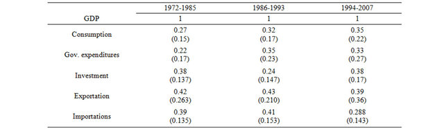
The results of the study of cyclical contributions of the variables of the GDP, thanks to the data from the Gabonese economy, can be viewed in Table 3 (Appendix 3).

The analysis of that table suggests the following observations:

1) Over the period studied, the cycle of the GDP seems to highlight three major phases representative of the main movements of the Gabonese economy: 1972-1985, 1986- 1993 and 1994-2007. The analysis of the contributions to the GDP cycles is based on three phases;

2) For the first phase, exports contribute about for 42% at the variance of the cycle of GDP. Then come imports and investments that respectively contribute to 39% and 38% to the variance of the cycle of the GDP. Finally, the contributions of the final consumption and government expenditure amount to 27% and 22%. Moreover, the values of standard gaps (between parentheses) indicate that exports constitute the GDP component whose amplitude of the cycle is the most important over this period. This result surprises a little because of the heavy weight of oil exports and significant fluctuations of the rates of this product on the international market, resulting from the oil shocks of 1973-1974 and 1979;

3) For the second phase, the contribution of exports (43%) is slightly greater than that of imports (41%). However, in terms of the fluctuation amplitude of the cycles of the different components of the GDP, Table 3 (Appendix 3) indicates the Government expenditure, records the highest value. Indeed, the evolution of this last variable is marked by strong fluctuations that confirm the dependence of the fiscal policy of Gabon to the receipts drawn from the exploitation and marketing of oil;

4) Finally, during the last phase, it seems that the changes observed are marked by the effects of the devaluation of the CFA franc in 1994. Indeed, if the contribution of the cycle of exports to the variance of the GDP cycle is always important, that of imports, however, becomes weak.

5. Conclusions

This article aimed to identify cycles of Gabon’s GDP and those of its main components (consumption, investment, government expenditure, exports and imports) and to study the interactions between them, namely the co-movements, degree of agreement and contributions to the variance of GDP.

Like [5,6], we identify cycles Gabon’s GDP and its components. Moreover, using the method of [13], we show that all the GDP variables are procyclical and there is a synchronization between the GDP cycle and those of its components. Finally, the contribution analysis, inspired by [14], suggests that the cycle of the variable relating to foreign trade, e.g. exports and imports, provide the most significant contributions to the variance of the GDP cycle.

However, the results must be nuanced. Indeed, the Gabonese economy is dependent on the evolution of oil prices, the results of this study could be refined by using a multivariate band-pass filter, as suggested by [15]. In particular, that methodology would take into account the unobserved components related to the endpoints effect and to the presence of a stochastic volatility that may affect Gabon’s GDP. This last aspect will be the subject of future research.

REFERENCES

Appendix 1: Graphs of Cycles

Appendix 2: Tables of Cycles Properties

GDP

Government expenditure

Imports

Exports

Investment in fixed capital

Final expenditure of consumption

Appendix 3: Interactions and Contributions

Table 1. Dynamic correlations.

Table 2. Correlation indices.

Table 3. Contribution of the GDP variables to the cyclicality of the GDP.

In parentheses. the values of standard deviations.

REFERENCES

- A. F. Burns and W. C. Mitchell, “Measuring Business Cycles,” National Bureau of Economic Research, Cambridge, 1946.
- S. Claessens, A. Kose and E. Terrones, “How Do Business and Financial Cycles Interact?” Research Department International Monetary, Washington DC, 2000.
- W. Hoffmaister, E. Roldos and P. Wickham, “Macroeconomic Fluctuations in Sub-Saharan Africa,” IMF Working Paper, 1997.
- P. Agenor, C. Mc Dermott and E. Prasad, “Macroeconomic Fluctuations in Developing Countries: Some Stylized Facts,” World Bank Economic Review, Vol. 14, No. 2, 2000, pp. 251-285. doi:10.1093/wber/14.2.251
- D. Corbae and S. Ouliaris, “Extracting Cycles from Nonstationary Data,” In: D. Corbae, S. Durlauf and B. Hansen, Eds., Econometric Theory and Practice: Frontiers of Analysis and Applied Research, Cambridge University Press, New York, 2006.
- J. Christiano and J. Fitzgerald, “The Band Pass Filter,” International Economic Review, Vol. 44, No. 2, 2003, pp. 435-465. doi:10.1111/1468-2354.t01-1-00076
- M. Baxter and R. King, “Measuring Business Cycles: Approximate Band-Pass Filters for Economic Time Series,” University of Virginia, Charlottesville, 1988.
- G. Bry and C. Boshan, “Cyclical Analysis of Time Series: Selected Procedures and Computer Programs,” UMI, Cambridge, 1971.
- D. Harding and A. Pagan, “Synchronization of Cycles,” Melbourne University, Parkville, 2000.
- R. Pagan, “Lecture 2: Measuring the Cycle,” IMF Lecture, New York, 2004.
- A. Haug and G. Dewald, “Longer-Term Effects of Monetary Growth on Real and Nominal Variables,” European Central Bank Working Paper, No. 382, 2004.
- W. K. Newey and K. West, “Automatic Lag Selection in Covariance Matrix Estimators,” Review of Economic Studies, Vol. 61, No. 4, 1994, pp. 631-653. doi:10.2307/2297912
- J. P. Allergret and A. Zantman. “Disentangling Business Cycles and Macroeconomic Policy in Mercusor: A VAR and Unobserved Components Model Approaches,” Observatoire Français de Conjoncture Economique.
- J. Stock and M. Watson, “Business Cycle Fluctuations in US Macroeconomic Time Series,” NBER Working Paper, 1998.
- J. Valle e Azevedo, “A Multivariate Band—Pass Filter for Economic Time Series,” Journal of the Royal Statistical Society Series C, Vol. 60, No. 1, 2011, pp. 1-301. doi:10.1111/j.1467-9876.2010.00734.x