Wireless Engineering and Technology
Vol.2 No.3(2011), Article ID:5829,9 pages DOI:10.4236/wet.2011.23025
Effect of Changes in Sea-Surface State on Statistical Characteristics of Sea Clutterwith X-band Radar
![]()
1Department of Communications Engineering, National Defense Academy, Yokosuka, Japan; 2Department of Intelligent Interaction Technology, University of Tsukuba, Tsukuba, Japan.
Email: reduan1786@gmail.com
Received March 9th, 2011; revised April 15th, 2011; accepted May 3rd, 2011.
Keywords: X-Band Radar, Sea Clutter, Significant Wave Height, Weibull Distribution, Log-Normal Distribution
ABSTRACT
We have made observations of X-band radar sea clutter from the sea surface and sea-surface state in the Uraga Suido Traffic Route, which is used by ships entering and leaving Tokyo Bay, and the nearby Daini Kaiho Sea Fortress. We estimated the distributions of reflected amplitudes due to sea clutter using models that assume Weibull, Log-Weibull, Log-normal, and K-distributions. We then compared the results of estimating these distributions with sea-surface state data to investigate the effects of changes in the sea-surface state on the statistical characteristics of sea clutter. As a result, we showed that observed sub-ranges not containing a target conformed better to the Weibull distribution regardless of Significant Wave Height (SWH). Further, sub-ranges conforming to the Log-Weibull or Log-normal distribution in areas contained a target when the SWH was large, and as SWH decreases, sub-ranges conforming to a Log-normal. We also showed that for observed sub-ranges not containing a target, the shape parameter, c, of both Weibull and Log-Weibull distribution correlated with SWH. The correlation between wave period and shape parameters of Weibull and Log-Weibull distribution showed a weak correlation.
1. Introduction
As electronics technology has advanced, equipment supporting marine navigation has become computerized, and highly automated vessels have begun to appear. Safe, reliable, and rapid goods delivery services are essential for a plentiful and comfortable society. To provide these services efficiently, cargo vessels are expected to increase in size, speed and energy efficiency, and ensuring the safe navigation of these vessels is an important issue. Sea charts are also essential for safe navigation, and Electronic Chart Display and Information Systems (ECDIS) [1] have been realized, able to display radar data overlaid on the charts. This has contributed to radar becoming essential for safe navigation of sea vessels.
The signal received by radar contains reflections from various objects besides the intended targets, such as land, clouds, rain, and the sea surface. All such undesired reflections from non-targets are referred to as clutter. The presence of this sort of clutter can result in false detection of targets or undetected targets, and is a major obstacle to target detection [2]. In order to suppress this clutter and detect targets accurately it is necessary to process the signals to obtain a Constant False Alarm Rate (CFAR), and to accomplish this, it is very important to study the statistical characteristics of clutter, such as the distribution of reflected amplitudes, in detail [2-8].
The reflected-clutter amplitude distribution differs depending on what type of objects create the reflection, and reflections from land are called ground clutter, from rain and clouds are called weather clutter, and from the sea surface are called sea clutter [2].
The amplitude of sea clutter reflections has been reported to increase in proportion to the height of the waves [9], but there have been no reports discussing how the statistical characteristics of sea-clutter reflection amplitudes are affected by statistical changes in the state of the sea surface. Sea-surface state is characterized by values such as wave period and Significant Wave Height (SWH), which is statistically close to visually observed wave heights. Accordingly, in this research we have taken observations of sea clutter and sea-surface state and compared them statistically to study the effects of sea-surface state on the statistical characteristics of sea clutter.
The paper is organized as follows: In Section 2, we indicate the observations which is included the sea state and the radar observations indicating the observation parameters. A solution to the sea clutter distribution assumptions and the distribution estimation are given in Section 3, and the effect on the reflected amplitude distribution by changes in the sea surface is discussed in Section 4.
2. Observations
We conducted observations of the sea-surface state at the same time as taking radar measurements. The radar observations were made in areas including the busy Tokyo Bay Uraga Suido Traffic Route and the Daini Kaiho Sea Fortress. The Daini Kaiho Sea Fortress is a fortification initially built on the water at the entrance to Tokyo Bay as part of the captial’s defenses, but it is now a facility for ensuring the safety of vessels passing through the Uraga Suido Traffic Route, with equipment such as lighthouses and beacons, and also instruments for measuring the sea state. The observations were taken between April 2, and December 3, 2010, including a total of 106 data points. Radar data obtained during rain was excluded from the study because it includes weather clutter from raindrops in addition to sea clutter. We also excluded data containing targets (ships, etc.) in the specified range where used for analyzing the statistical characteristics of sea clutter. We then assigned an observation number to each of the remaining 65 data points used for the study.
2.1. Sea State Observations
Significant wave height (SWH) and wave period data was extracted from ocean wave and the significant wave state data at the Tokyo Bay Daini Kaiho Sea Fortress from the National Ocean Wave information network for Ports and HArbourS (NOWPHAS) [10].
2.2. Radar Observations
The region was observed using X-band radar equipment installed on the roof top at the National Defense Academy in Yokosuka City. The main parameters of the Xband radar are given in Table 1. Figure 1 has an aerial photograph of the area around Tokyo Bay Uraga Suido Traffic Route showing the approximate region of the radar images taken as observation data with a dashed line. The extracted data covered an azimuth range sweep of 355.5˚ to 18.0˚ and distance range from 4.0 to 6.0 km, in the Uraga Suido Traffic Route surrounding the Daini
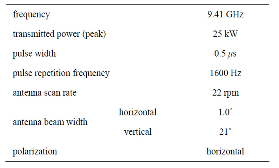
Table 1. X-band radar parameters.
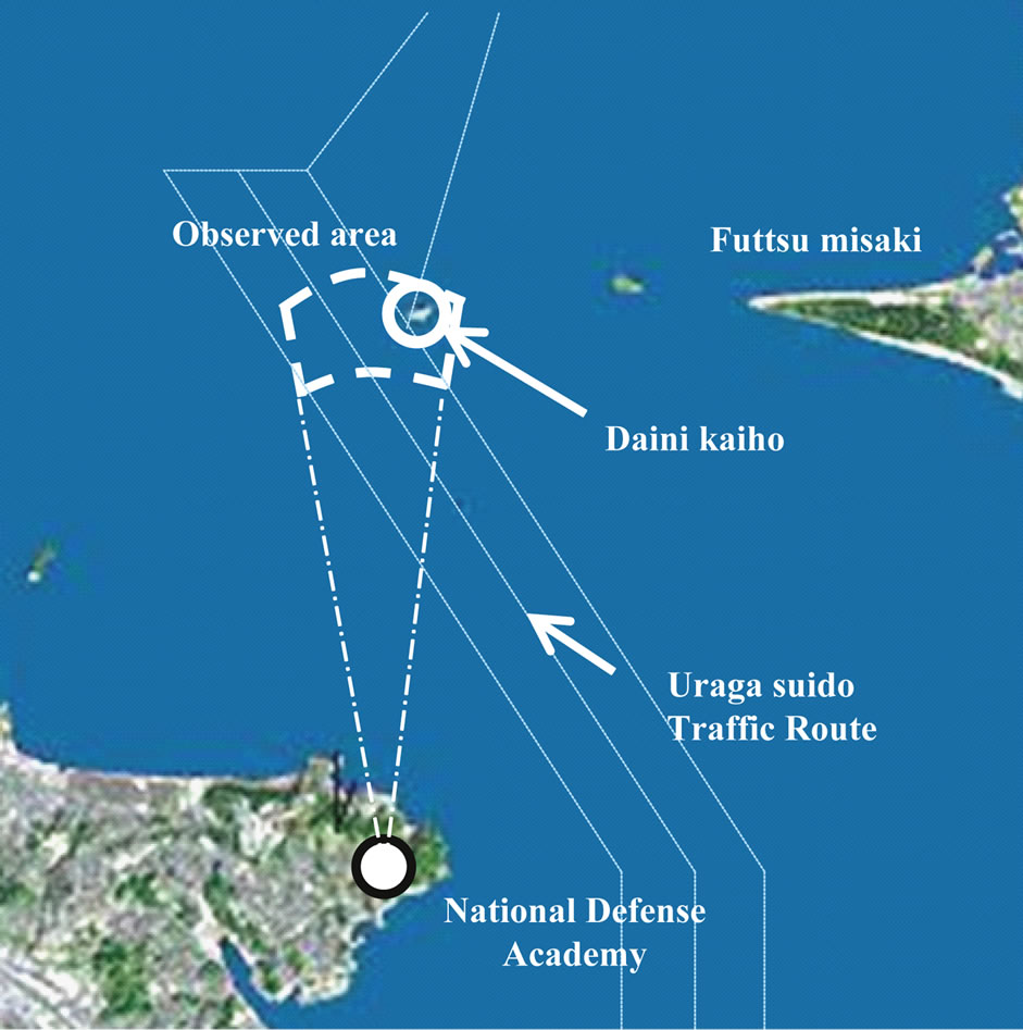
Figure 1. Observed area.
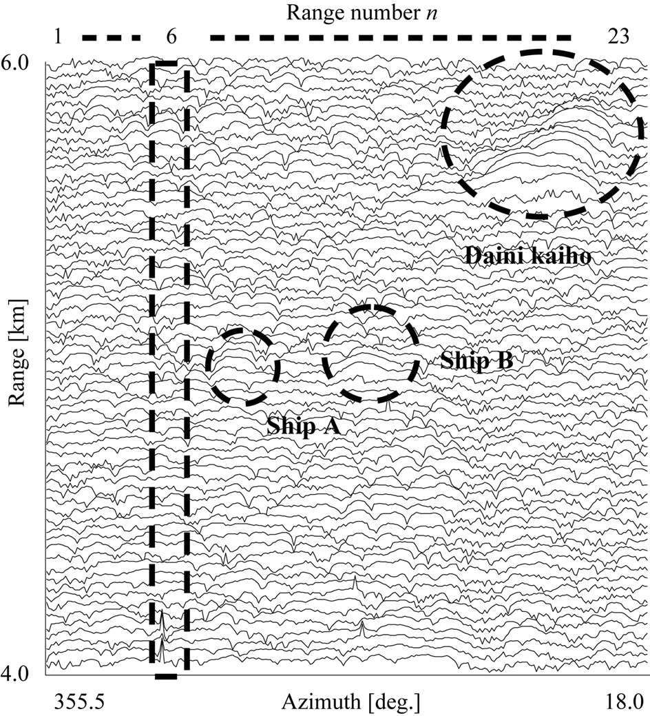
Kaiho Sea Fortress. 273 sweeps of the azimuth range were made. The antenna is installed 90 m above sea level, so the grazing angle was 1.4˚. 256 points on each of the range and azimuth axes were taken, totaling 65,536 data points, and the reflection amplitude at each point was quantized to 256 levels, from 0 to 255. As examples of this observed data, data from when the SWH was high (1.27 m) is shown in Figure 2(a) (observation number 64, Dec. 3), and when the SWH was low (0.21 m) is shown in Figure 2(b) (observation number 21, Apr. 26). When estimating the amplitude distribution of the reflected signals the data was divided in the azimuth direction into 23 ranges, each equivalent to the horizontal beam width of the radar antenna, and a range number, n, was assigned to each of them. The range shown with a dashed line (n = 6) was used to analyze the effects of SWH on the reflected wave distribution. This range is near the center of the Uraga Suido Traffic Route, with few entering
 (a)
(a)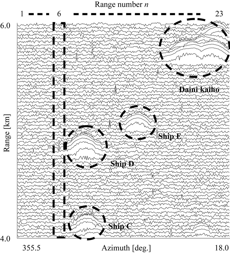 (b)
(b)
Figure 2. Observed data. (a) Significant wave height of 1.27 m; (b) Significant wave height of 0.21 m.
and leaving vessels passing through it and no reflective objects other than waves. The bump shapes shown surrounded by circles are radar targets: vessels passing through the Uraga Suido Traffic Route (Ships A to E) and the Daini Kaiho Sea Fortress.
3. Clutter Distribution Assumptions
We then tested conformity to the assumed distributions using the observation data for when the SWH was large and small, as shown in Figure 2(a) and (b) respectively.
Reference [11] gives a method for estimating parameters for a random variable according to various distributions as well as the expected values. In this study, we estimated the parameters using a maximum likelihood estimator.
3.1. Assumed Distribution Models
Sea clutter reflection amplitude distributions have been reported to follow K, Weibull, Log-Weibull, and Lognormal distributions [12], and these have all been studied for use in implementing CFAR [2]. However, there is a known problem [12] with the K-distribution, which is expressed in terms of shape (v) and scale (h) parameters. When sections of the reflected clutter amplitude probability are large, and get larger than a Raleigh distribution (a Weibull distribution with shape parameter of 2), the value of v goes to infinity and it is not possible to calculate the probability density. Thus, when assuming a K-distribution model it was not possible to estimate the distribution for sub-ranges not containing a target, regardless of the SWH, as is shown by the error marks in Tables 2 and 3.
A Weibull distribution can be expressed by the following probability density function.
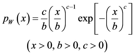 (1)
(1)
The Log-Weibull distribution is expressed by the following probability density function.
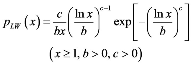 (2)
(2)
where, x is the reflected amplitude, b is the scale parameter and c is the shape parameter.
The Log-normal distribution is given by the following probability density function.
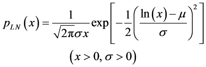 (3)
(3)
where, μ is the mean and σ is the standard deviation.
The K-distribution is given by the following probability density function.
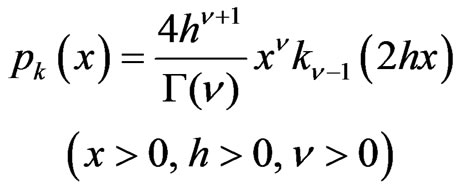 (4)
(4)
where, kν-1 is a modified Bessel function, and its parameters are a scale parameter, h, and a shape parameter, ν.
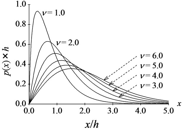
For reference, Figure 3(a) shows the changes in the shape of the Weibull distribution when b is fixed and the shape parameter, c, is varied, Figure 3(b) shows how the Log-normal distribution changes when the mean, μ, is fixed and the standard deviation, σ, is varied, and Figure 3(c) shows how the K-distribution changes when the scale parameter, h, is fixed and the shape parameter, v, is varied.
The Log-Weibull distribution is positioned between the Weibull and Log-normal distributions [2].
As the highest parts of the reflected clutter amplitude get higher, the Weibull and Log-Weibull distributions tend toward those with higher shape parameter (c) values, and the Log-normal distribution toward shapes with a smaller standard distribution, σ.
3.2. Beam Width and Sub-Ranges
It is generally thought that reflected radar signals are strongly correlated within the antenna beam width, and have similar characteristics [2]. Thus, we divided the
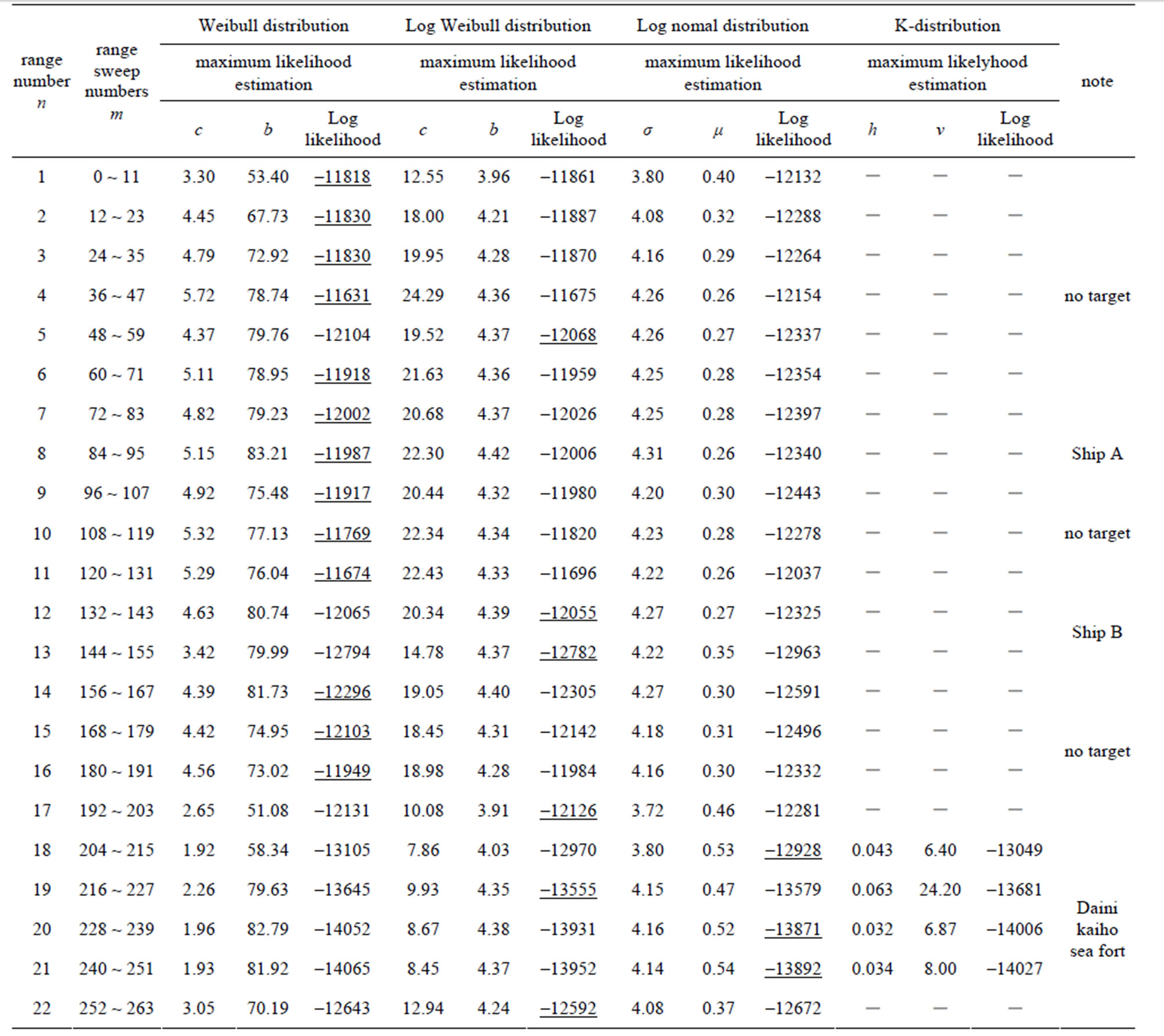
Table 2. Result of distribution estimation for different range numbers at significant wave height of 1.27 m (observation number 64).
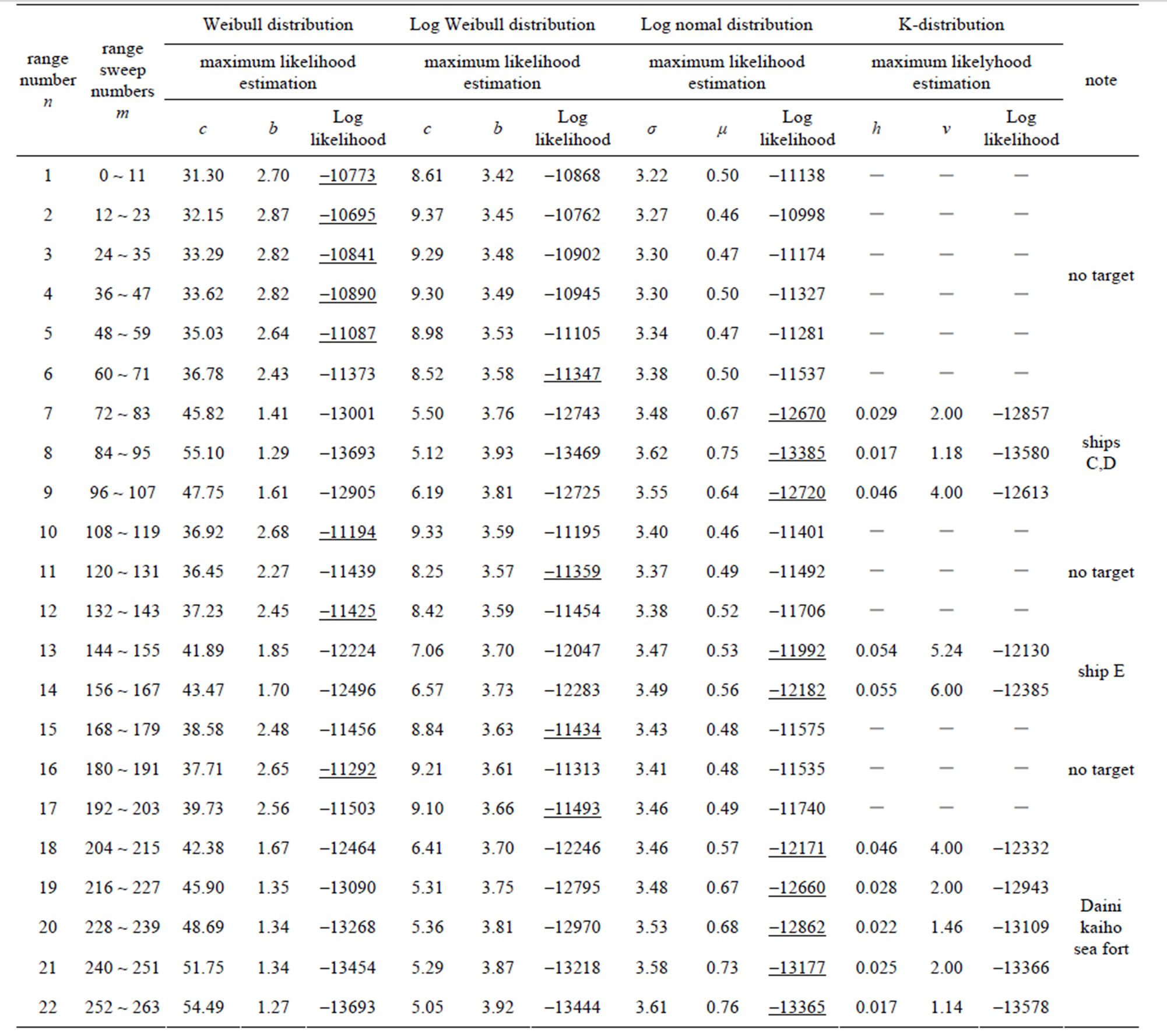
Table 3. Result of distribution estimation for different range numbers at significant wave height of 0.21 m (observation number 21).
 (a)
(a)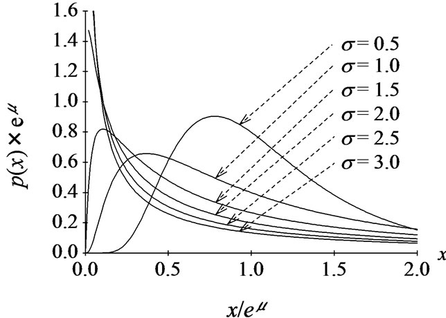 (b)
(b) (c)
(c)
Figure 3. Shape of Weibull distribution, Log-normal distribution and K-distribution. (a) Weibull distribution; (b) Log-normal distribution; (c) K-distribution.
observed data into 22 sub-ranges equivalent to the horizontal antenna-beam width and tested conformity to the assumed distributions in each of the sub-ranges. The number of range sweeps, m, is given by the following equation, and 1.0 degrees of horizontal antenna beam width is equivalent to 12 sweeps (m = 12).
 (5)
(5)
where,  is the pulse repetition frequency,
  is the horizontal antenna beam width, and
  is the antenna scan rate.
3.3. Conformity Testing
To test the conformity of the observed data to the assumed distribution models, we used log-likelihood.
Models with higher logarithmic likelihood can be judged to be better conforming [11].
3.4. Logarithmic Likelihood
Reference [13] gives a method for the log-likelihood algorithm to test the conformity estimating.
First we assume that the true probability distribution  is known. Here
  is the probability that the nth event occurs. Next we will consider a sufficiently large number of trials. Then the nth event will occur approximately m =
  times. As a model, we assume the probability distribution
 . By observing the M samples obeying this distribution, the probability W is written as
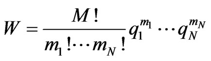 (6)
(6)
Here W is the probability that we obtain the probability distribution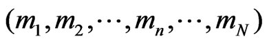 . By taking a logarithm of both sides of Equation (6) and dividing by M, we obtain
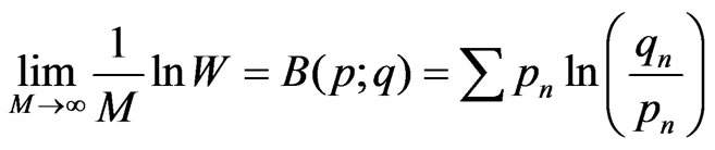 (7)
(7)
where  is called the Kullback-Leibler entropy [14]. From the above discussion, the probability is that the predicted distribution realized becomes large with larger values of B. In this sense, B is used as a model estimation, i.e. the larger values of B mean a good model.
The Kullback-Leibler entropy is rewritten as
 (8)
(8)
The second term on the right-hand side depends only on a true distribution. On the other hand, only the first term plays an important role in estimating the model. This term is interpreted as an expected value of . Therefore, if a probability distribution is given by
  with
with  the log-likelihood divided by M is given by
 (9)
(9)
As M is increased indefinitely, Equation (9) converges to the average log-likelihood. We can write
 (10)
(10)
Then Equation (9) is the same as Equation (10) which is multiplied by . The first term in Equation (8) is estimated from the M numbers of the observed values
  Then the logarithmic likelihood L is defined as
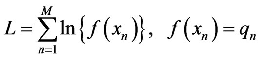 for
for  (11)
(11)
Here a function  is a probability that the observed values are x, and depends on the model. The larger L is the better model.
3.5. Distribution Estimation Results
The results of estimating distributions and the log likelihood of each are shown in Tables 2 and 3. The distribution that is most conforming for each sub-range is underlined in the column of Log likelihood. Entries where the distribution could not be estimated are shown with a dash (‘-’). The number of samples for each range is 3072.
From the results of estimating distributions, for subranges not containing ships, the Sea Fortress, or other non-wave reflective objects, the sea clutter amplitude distributions conformed to the Weibull distribution regardless of whether the SWH was high or low. For subranges containing strong reflections from targets and other non-wave objects, ranges where they cause strong reflections clearly conform better to the Log-Weibull and Lognormal distributions, whose probability density distribution curves have long tails. This tendency is particularly striking when the SWH is low. This shows that, regardless of whether the sea clutter reflected amplitude distribution is a Weibull distribution or not, the presence of the target prevents adequate estimation of the distribution. This result shows that threshold-detection CFAR cannot be done accurately, because it sets an amplitude threshold based on the results of estimating the distribution and attempts to detects targets while maintaining a constant false-alarm rate [2,3].
As an example of estimation for the ranges containing no target, the observation data for range number 6 (n = 6) and graphs of probability distributions using the coefficients calculated by maximum-likelihood estimation are shown in Figure 4. The vertical axis is the probability, and the horizontal axis shows the amplitude of the reflected signal. The line-segment graph is the reflectedsignal-amplitude observed data, and the curved lines are the probability density distributions. This confirms, even visually, that for ranges where there is no target the Weibull distribution corresponds better to the data regardless of whether the SWH is high or low.
4. Effect on the Reflected Amplitude Distribution by Changes in the Sea Surface
In order to investigate how changes in the state of the sea surface affect the statistical characteristics of sea clutter, we analyzed the correlation between the SWH and wave period and the parameters calculated from the distribution estimation, for the 65 observation data sets under
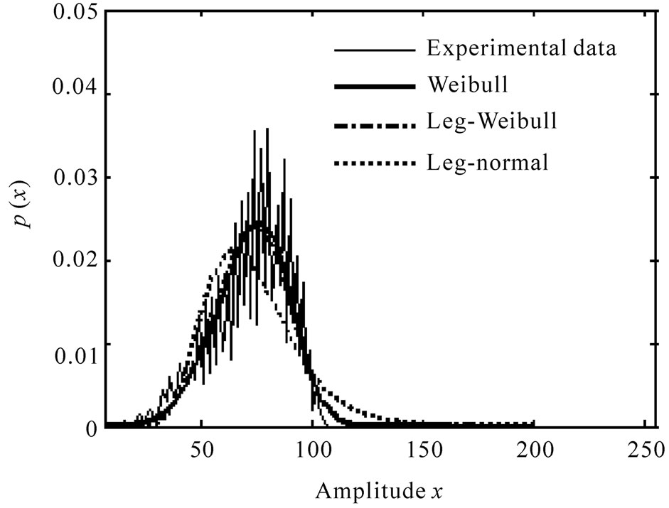 (a)
(a)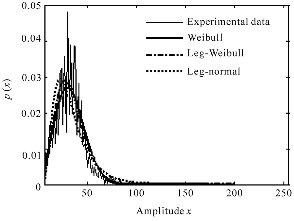 (b)
(b)
Figure 4. Result of distribution estimation for range number 6. (a) Significant wave height of 1.27 m; (b) Significant wave height of 0.21 m.
study and the range with no reflective objects other than waves (range no. n = 6).
4.1. Sea Surface Changes
Changes in the height and period of significant waves during the observation period are shown in Figure 5. The horizontal axis shows the observation numbers assigned to each observation in order. The results show SWH ranging from 0.21 to 1.27 m and wave period ranging from 3.1 to 5.1 s.
4.2. Sea Surface and Estimated Parameter Changes
How the parameters of each distribution changed as the state of the sea surface changed is shown in Figure 6. The horizontal axis shows observation number, while the vertical axis shows the Weibull distribution shape parameter, c, the Log-Weibull distribution shape parameter, c, and the Log-normal distribution standard deviation, σ. As the state of the sea surface changed, the shape parameter, c, of the Weibull distribution fluctuated between 1.74 and 6.38, that of the Log-Weibull between 6.38 and 28.17, and the standard deviation, σ, of the Log-normal distribution ranged from 0.214 to 0.576.
4.3. Relation between SWH and Estimated Parameters
The correlations between the SWH and the shape parameter, c, for the Weibull distribution, which conformed better when the SWH was both high and low, and the Log-Weibull distribution, are shown in Figure 7. From this we see that the shape parameter, c, for the Weibull distribution had a correlation coefficient of 0.755, and for Log-Weibull distribution it was 0.794, so the Log-Weibull distribution showed a stronger correlation.
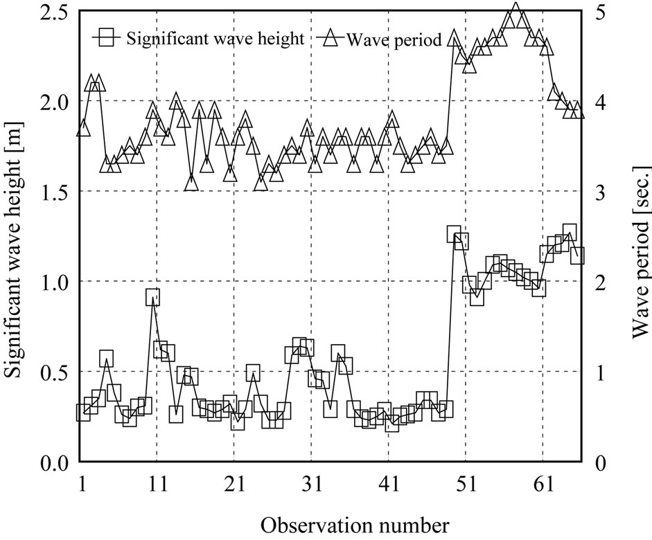
Figure 5. Observed sea condition.
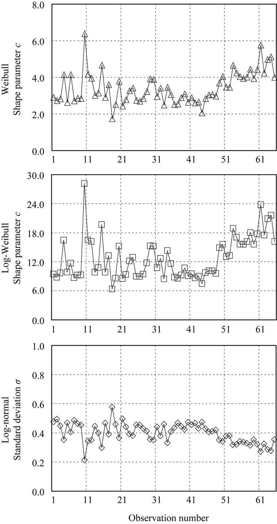
Figure 6. Variation of estimated distribution.
4.4. Relation between Wave Period and Estimated Parameters
The correlation between wave period and the shape parameter, c, for the Weibull and Log-Weibull distributions are shown in Figure 8. The correlation coefficient for the Weibull shape parameter, c, is 0.436, and for the LogWeibull distribution it is 0.499, so both are only weakly correlated.
5. Conclusions
We made observations of the sea clutter using X-band radar and the state of the sea surface in the area of the Uraga Suido Traffic Route, where vessels enter and leave Tokyo Bay, including the Daini Kaiho Sea Fortress. We

Figure 7. Correlation between significant wave height and estimated distribution.
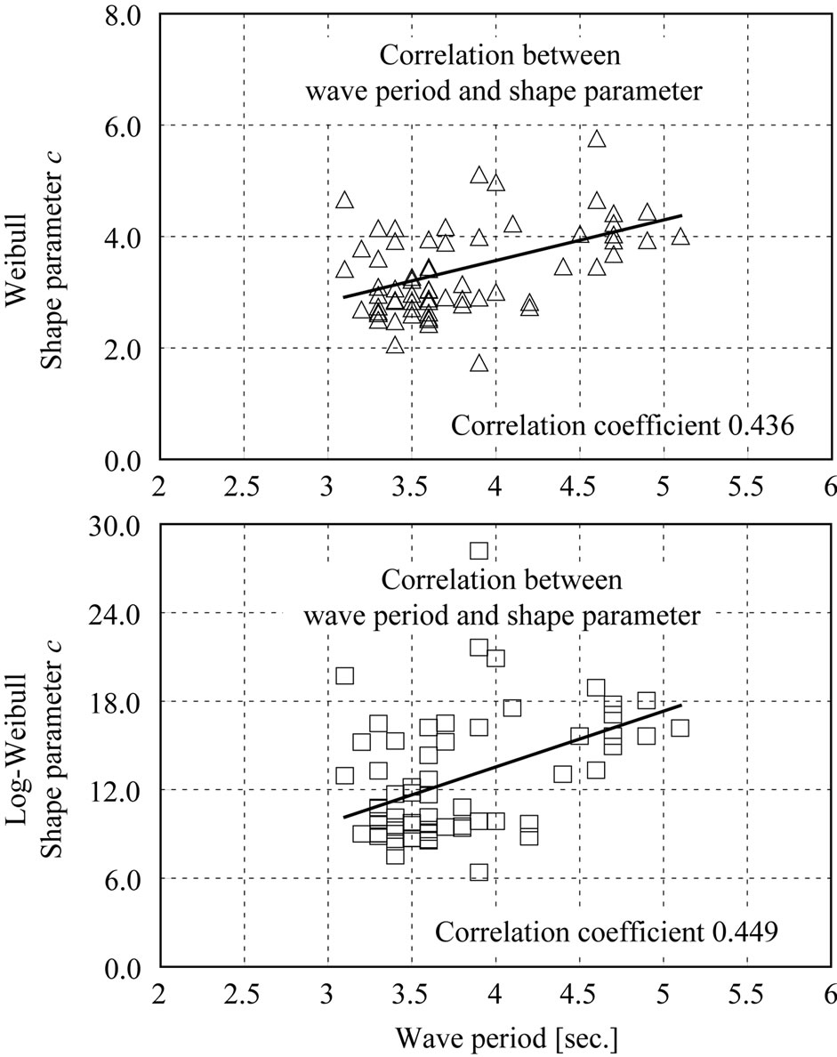
Figure 8. Correlation between wave period and estimated distribution.
estimated the distribution of the sea clutter reflected amplitudes using Weibull, Log-Weibull, Log-normal and K-distribution models. We then compared the results of estimating the distributions with the sea-surface state data and studied the effects of changes in sea state on the statistical characteristics of the sea clutter.
As a result, ranges not containing a target conformed better to the Weibull distribution regardless of SWH, but observed ranges containing a target conforming more to the Log-Weibull distribution when the SWH was high, and conformed to a Log-normal distributions when the SWH was low. Also, for observed ranges not containing a target, SWH and the shape parameter, c, of the Weibull distribution correlated with correlation coefficient of 0.755, and for the Log-Weibull distribution this figure was 0.794. The correlation between wave period and Weibull distribution shape parameter, c, had a coefficient of 0.436, and for the Log-Weibull distribution, the coefficient was 0.449, so both were only weakly correlated to wave period.
In the future, it will be necessary to study new threshold detection CFAR methods that detect targets more accurately by setting thresholds using the distribution estimation results we have studied, and also to examine the use of SWH and other approaches to setting thresholds.
REFERENCES
- International Meteorological Organization Resolution A.817 (19), “ECDIS Performance Standards,” 2000.
- M. Sekine, “Radar Signal Processing Techniques,” The Institute of Electronics, Information and Communication Engineers, Tokyo, 1991.
- M. L. Skolnik, “Introduction to Radar System,” McGrawHill, New York, 1982.
- J. Croney, “Clutter on Radar Displays,” Wireless Engineering, Vol. 33, 1956, pp. 83-96.
- M. Sekine, T. Musha, Y. Tomita, T. Hagisawa, T. Irabu, E. Kiuchi, “On Weibull-Distributed Weather Clutter,” IEEE Transactions on Aerospace and Electronic Systems, Vol. AES-15, No. 6, 1979, pp. 824-830. doi:10.1109/TAES.1979.308767
- M. Sekine and Y. Mao, “Weibull Radar Clutter,” Peter Peregrinus Ltd., London, 1990.
- M. Sekine, T. Musha, Y. Tomita and T. Irabu, “Suppression of Weibull-Distributed Clutters Using a Cell-Averaging LOG/CFAR Receiver,” IEEE Transactions on Aerospace and Electronic Systems, Vol. AES-14, No. 5, 1978, pp. 823-826. doi:10.1109/TAES.1978.308637
- M. Sekine, T. Musha, Y. Tomita, T. Hagisawa, T. Irabu and E. Kiuchi, “Suppression of Weibull-Distributed Weather Clutter,” Proceedings of IEEE International Radar Conference, New York, 1980, pp. 294-298.
- P. Z. Peebles Jr., “Radar Principles,” John Wiley and Sons Inc., New York, 1998.
- Ministry of Land, Infrastructure, Transport and Tourism of Japan, “NOWPHAS, Nationwide Ocean Wave Information Network for Ports and HArbourS,” 2010. http://www.mlit.go.jp/kowan/nowphas/index.html
- N. L. Johnson, S. Kotz and N. Balakrishnan, “Distributions in Statistics: Continuous Univariate Distributions,” Wiley Series in Probability and Mathematical Statistics, 2nd Edition, Vol. 1, 1994.
- S. Sayama, S. Ishii and M. Sekine, “Amplitude Statistics of Sea Clutter Observed by L-band Radar,” IEEE Transactions on Fundamentals and Materials, Vol. 126, No. 6, 2006, pp. 426-429. doi:10.1541/ieejfms.126.426
- Y. Sakamoto, M. Ishiguro and G. Kitagawa, “Information Statistics,” Kyoritsu Syuppan Co., Ltd., Tokyo, 1983.
- S. Kullback and R. A. Leibler, “On Information and Sufficiency,” Annals of Mathematical Statistics, Vol. 22, No. 1, 1953, pp. 79-86. doi:10.1214/aoms/1177729694