Energy and Power Engineering
Vol. 4 No. 5 (2012) , Article ID: 22847 , 8 pages DOI:10.4236/epe.2012.45049
Probabilistic Assessment of Power System Performance Quality
SEC Chair in Power System Reliability and Security, King Saud University, Riyadh, KSA
Email: melkady@ksu.edu.sa
Received July 19, 2012; revised August 20, 2012; accepted September 2, 2012
Keywords: Power Systems; Probabilistic Analysis; Reliability; Quality Assessment; Linear Programming
ABSTRACT
In a recently published work by the authors, a novel framework was developed and applied for assessment of reliability and quality performance levels in real-life power systems with practical large-scale sizes. The new assessment methodology is based on three metaphors (dimensions) representing the relationship between available generation capacities and required demand levels. The developed reliability and performance quality indices were deterministic in nature. That is, they represent one operating state (a snapshot of the system conditions) in which the required demand as well as the generation and transmission capacities are known with 100% certainty. In real life, however, load variations occur randomly so as the contingencies which cause some generation and/or transmission capacities to be lost (become unavailable). In other words, neither the load levels nor the generation or transmission capacities are known with absolute certainty. They are rather subject to random variations and, consequently, the calculated reliability and performance quality indices are all subject to random variations where only expected values of these indices can be evaluated. This paper presents a major extension to the previously published work by developing a theory and formulas for computing the expected values of different system reliability and performance quality indices. In this context, a “contingency scenario” or a system “demand level” are regarded, in a more general sense, as a “state”, which occurs with certain probability and represents a given demand value and availability pattern of various capacities in the system. The work of this paper provides a practical and meaningful methodology for real-life assessment of power system reliability and performance quality levels. Practical applications are also presented, for demonstration purposes, to the Saudi electricity power grid.
1. Introduction
Maintaining a continuous and sufficient power supply to the customers at a reasonable cost is the prime objective of electric power companies around the world. In this regard, power system cost-effectiveness, security, adequacy and reliability analyses have become a major concern in today’s highly-competitive business environment of power utility planning and operations [1-3]. In a recent paper by the authors [4], a novel framework was developed and applied for assessment of reliability and quality performance levels in real-life power systems with practical largescale sizes. The new assessment methodology is based on three metaphors (dimensions) representing the relationship between available generation capacities and required demand levels. The first metaphor defines whether or not the capacity exists, the second metaphor defines whether or not the capacity is needed, and the last metaphor defines whether or not the capacity can reach (delivered to) the demand. The eight possible combinations associated with the 0/1 (Yes/No) values of the three metaphors would, in turn, define a set of powerful systemwide performance quality measures relating to generation deficiency, redundancy, bottling, etc. The developed reliability and performance quality indices were deterministic in nature. That is, they represent one operating state (a snapshot of the system conditions) in which the required demand as well as the generation and transmission capacities are known with 100% certainty.
In real life, however, load variations occur randomly so as the contingencies which cause some generation and/or transmission capacities to be lost (become unavailable). In other words, neither the load levels nor the generation or transmission capacities are known with absolute certainty. They are rather subject to random variations and, consequently, the calculated reliability and performance quality indices are all subject to random variations where only expected values of these indices can be evaluated.
Methods for computing probabilistic contingency-based reliability and performance quality indices have previously been published in the literature [5-7]. These methods are based on a combined contingency analysis and reliability evaluation scheme which integrates both the contingency effect and its probability of occurrence into one routine of analysis. In the present research work, similar analysis will be used to compute the expected values of different system reliability and performance quality indices. In this context, a “contingency scenario” or a system “demand level” are regarded, in a more general sense, as a “state”, which occurs with certain probability and represents a given demand value and availability pattern of various capacities in the system.
The work of this paper presents a major extension to the previously published work [4] by developing a theory and formulas for computing the expected values of different system reliability and performance quality indices. In this context, a “contingency scenario” or a system “demand level” are regarded, in a more general sense, as a “state”, which occurs with certain probability and represents a given demand value and availability pattern of various capacities in the system.
The work of this paper provides a practical and meaningful methodology for real-life assessment of power system reliability and performance quality levels. Practical applications are also resented in the Saudi electricity power grid.
2. Power System Quality Assessment
2.1. Performance Quality Framework
In the framework presented in [4], three metaphors (dimensions) were introduced to represent the relationship between certain system generation capacity and the demand. These metaphors relate to the following demand fulfillment issues:
1) Need of capacity for demand fulfillment;
2) Existence of capacity (availability for demand fulfillment);
3) Ability of capacity to reach the demand.
The first metaphor defines whether or not the capacity is needed, the second metaphor defines whether or not the capacity exists, and the last metaphor defines whether or not the capacity can reach (delivered to) the demand. The eight possible combinations associated with the 0/1 (Yes/No) values of the three metaphors would, in turn, define a set of powerful system-wide performance quality measures, namely:
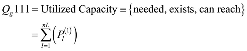
1) Utilized: A given capacity is said to be utilized if it is needed (for demand fulfillment), exists, and can reach the demand;
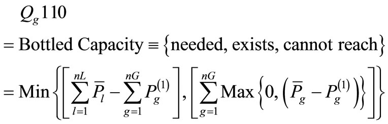
2) Bottled: A given capacity is said to be bottled if it is needed (for demand fulfillment) and exists, but cannot reach the demand;
3) Shortfall: A given capacity is said to be shortfall if it is needed (for demand fulfillment) and, anyhow, does not exist and can reach the demand;
4) Deficit: A given capacity is said to be deficit if it is needed (for demand fulfillment) but, however, does not exist and cannot reach the demand;
5) Surplus: A given capacity is said to be surplus if it is not needed (for demand fulfillment) although exists and can reach the demand;
6) Redundant: A given capacity is said to be redundant if it is not needed (for Demand fulfillment) although exists but, anyhow, cannot reach the demand;
7) Spared: A given capacity is said to be spared if it is not needed (for demand fulfillment) and, anyhow, does not exist although can reach the demand;
8) Saved: A given capacity is said to be saved if it is no needed (for demand fulfillment) and, anyhow, does not exist and cannot reach the demand.
We note here that the above performance quality measures are associated with different combinations (topples) of the three quality metaphors, namely, “existence”, “need” and “ability to reach the demand”. The corresponding quality state of a given capacity can be represented by a threevalue expression of either a “Yes/No” or “1/0” type indicating the true/false value associated with each quality metaphor.
The evaluation of the above quality indices requires the knowledge of the following data types for the demand and various system facilities:
1) The value of demand required to be supplied;
2) The value of generation capacity as well as the maximum site capacity (the limit of potential increase in existing generation capacity);
3) The value of transmission capacity.
2.2. Linear Program Formulation
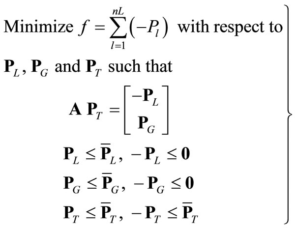
In the computational scheme of [4], the integrated system quality assessment is performed via solving a master linear programming problem [8] in which a feasible power flow is established which minimizes the total system non-served load subject to capacity limits and flow equations. The master linear program, which utilizes the network bus incidence matrix A, is formulated as
 (1)
(1)
In the above master linear program,
 = vector of nT elements representing transmission branch capacities;
 = vector of nL elements of peak bus loads;
 = vector of nG elements representing generator capacities.
Also, in the above master linear program (1), PL, PG, and PT are nL, nG and nT column vectors representing the actual load bus powers (measured outward), generator bus powers (measured inwards) and transmission line powers (measured as per the network bus incidence matrix A), respectively. The solution of the above linear program provides a more realistic (less conservative) flow pattern in view of the fact that when load curtailments are anticipated, all system generation resources would be re-dispatched in such a way which minimizes such load cuts. The feasible flow pattern established from the Master Linear Program is then used to evaluate various integrated system quality indices through a set of closely related sub-problems.
2.3. Implementation Mechanisms
For real life power systems with practical sizes, the quality indices cannot be evaluated by inspection. An appropriate computerized scheme is needed in order to properly evaluate various quality indices according to their stated definitions. The master linear program presented before forms the bases for analyzing and evaluating the quality indices. For example, the Load Supply Reliability can be evaluated as follows:

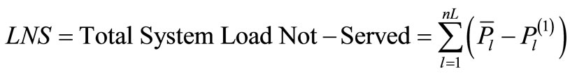
where the bus loads at the solution of the master linear program are termed as , and Pl denotes the solution load value at bus (l).
On the other hand, generation quality indices are defined in terms of the previously defined “1/0” states indicating the (Needed, Exists, Can-reach) true/false values associated with each quality metaphor. We shall use the symbol Qgijk to indicate the generation quality index state. Also, in the following expressions, we shall use Min{x, y, ···, z} to indicate the minimum of x, y, ···, z. The notation
Similarly, the Bottled Generation Capacity index is given by
Also, the Surplus Generation Capacity (Qg011) is calculated as
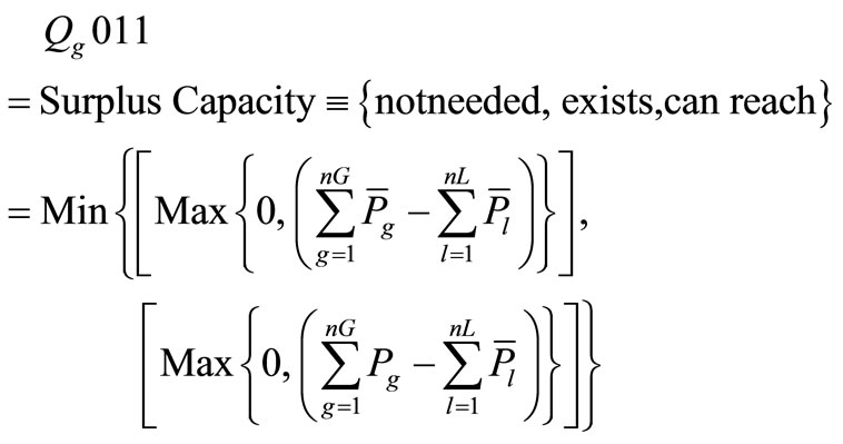
where the generation output values Pg are calculated at the solution of the linear program with open limits on the loads.
3. Probabilistic Assessment
3.1. Probabilistic Reliability Indices
The power system can be described, for the purpose of composite reliability and performance quality assessment, by the three-component model, as shown in Figure 1, in which generation, transmission and load are considered as multi-state elements of the power system.
For a given operating state m, the values of the network variables will be the solution of the maximum load-supply optimization problem described in the previous section. Also, let fm be the probability of operating state m (the sum of fm for all m, including base-case scenario is 1). Then, the following three system-wide reliability indices may be defined:
1) Loss of Load Probability
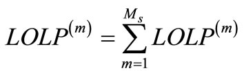 (2a)
(2a)
where
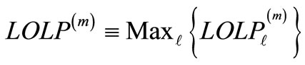 (2b)
(2b)
represents the system loss of load probability for any operating state m (load level, loss of generation and/or transmission capacities) in the power grid,
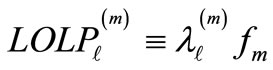 (2c)
(2c)
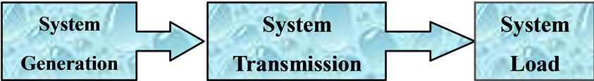
Figure 1. System model reliability evaluation.
represents the loss of load probability at bus l for operating state m,
 (2d)
(2d)
and  denotes the scheduled (required) load at load bus l. Also, in Equation (3.8), Ms denotes the number of all possible states.
2) Expected Load Not-Served
 (3a)
(3a)
where nL is the number of load buses in the system,
 (3b)
(3b)
represents the expected value of load not-served at bus l,
 (3c)
(3c)
represents the expected value of Load Not-Served at bus l for the operating state m, and

which is obtained from the solution of the Master Linear Program (1).
3) Expected Energy Not Served
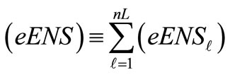 (4a)
(4a)
where
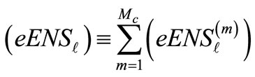 (4b)
(4b)
 (4c)
(4c)
represents the expected value of energy not served at a bus l, and
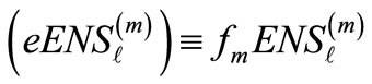 (4d)
(4d)
represents the expected value of energy not served at bus l for operating state m,
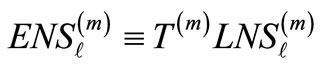 (4e)
(4e)
represents the energy not served at bus l for operating state m, and T(m) denotes the time duration of operating state m.
3.2. Probabilistic Performance Quality Indices
Probabilistic performance quality indices can be calculated using the previously derived formulas based on the solution of the master linear program (1) subject to random variations of system demand level as well as forced outages in various generation and transmission facilities.
For example, the load variations, which are accounted for using the so-called “load-duration curves” can be used to calculate the expected value of the Load Not-Served (LNS), which is widely known as the Expected Load NotServed (eLNS).
On the other hand, the randomness in the generation and transmission capacity availability are accounted for using the so-called forced-outage rates (or availability rates) associated with various facilities. Consequently, the expected values of the performance quality indices Qg111, Qg110, Qg101, etc., denoted by eQg111, eQg110, eQg101, etc., can be evaluated using the modeled randomness of the system load as well as the generation and transmission capacity availabilities.
4. Applications to SEC Power System
4.1. SEC Quality Performance Indices
In a recently completed industry supported study, applications were conducted on a practical power system comprising a portion of the interconnected Saudi power grid. The power system consists of two main regions, namely the Central region and the Eastern region. The two systems are interconnected through two 380 kV and one 230 kV double-circuit lines. Four zones are identified in the present analysis, three in the Central region (Riyadh, Qassim and Hail zones) and one in the Eastern region. In this application, three reliability and quality performance indices are considered, namely the system Load Not-Served (LNS), Utilized Generation Capacity (Qg111) and the Bottled Generation Capacity (Qg110). In the present work, a particular focus will be on Qassim and Hail zones for demonstration purposes. The system models used for these two zones are shown in Figures 2(a) and (b), respectively. Table 1 outlines the network data in terms of generation and transmission facilities as well as system loads. Figures 3(a) and (b), on the other hand, summarize the results of the performance quality measures applied to the SEC power system for various system status (isolated or connected) of each zone.
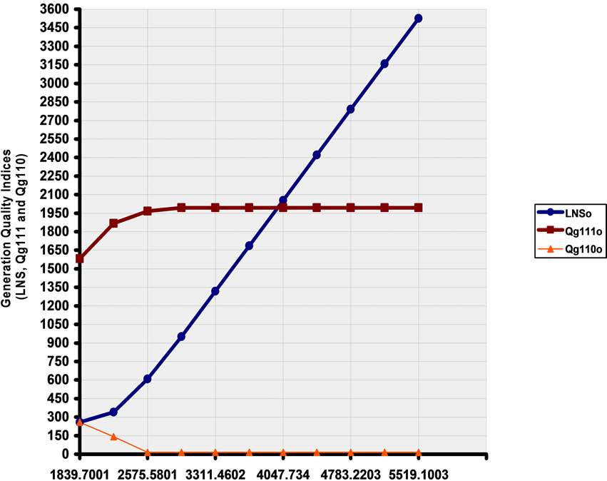
In particular, Figures 3(a) and (b) depict the variation of the variation of quality indices (LNS, Qg111 and Qg110) with the required load level of the Qassim isolated and interconnected network, respectively.
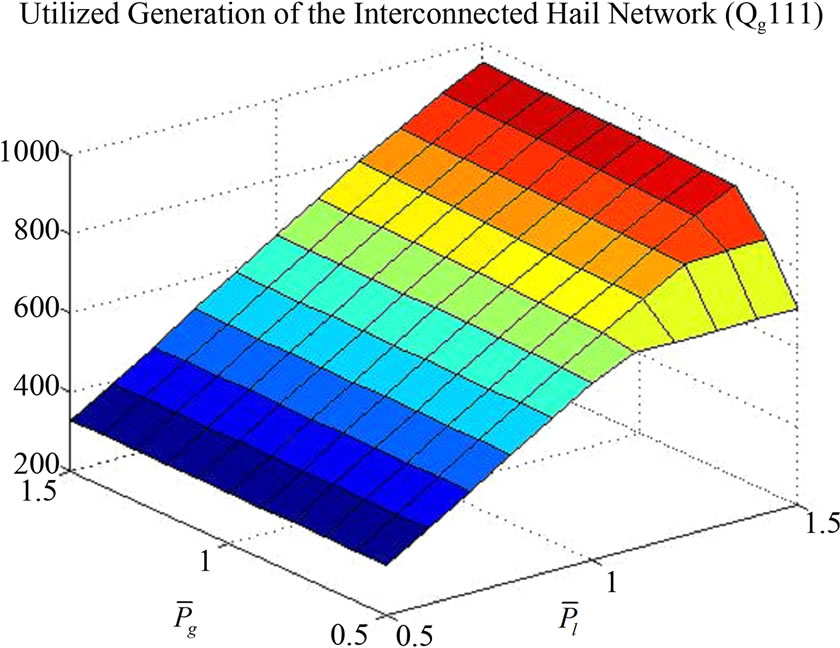
Figures 4(a) and (b), on the other hand, show 3-dimensional graphs depicting the variation of Utilized Generation Capacity index Qg111 with both load and generation capacity levels of the Hail isolated and interconnected network, respectively.
The results obtained reveal several important observations. For example, the results obtained for the isolated network scenario of Qassim zone (Figure 3(a)) show that the Load Not-Served is non-zero even for relatively low
 (a)
(a) (b)
(b)
Figure 2. (a) Single-line diagram of SEC—qassim zone; (b) Single-line diagram of SEC—hail zone.
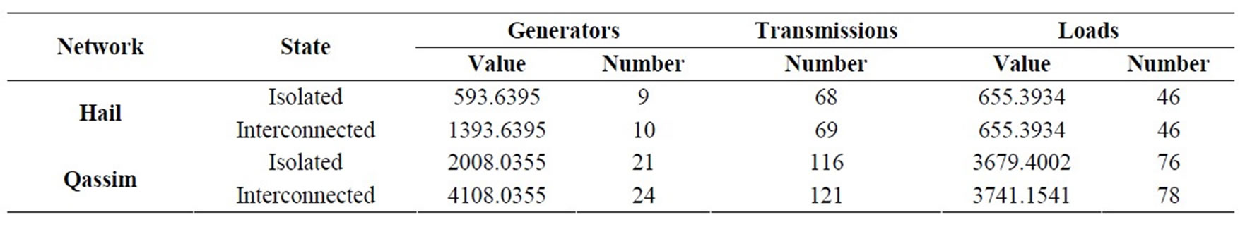
Table 1. Generation, transmission and loads of SEC power system.
 (a)
(a)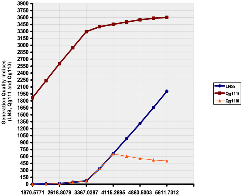 (b)
(b)
Figure 3. (a) Variation of quality indices (LNS, Qg111 and Qg110) with the required load level of the qassim isolated network; (b) Variation of quality Indices (LNS, Qg111 and Qg110) with the required load level of the qassim interconnected network.
 (a)
(a) (b)
(b)
Figure 4. (a) 3-dimensional graph showing variation of utilized generation index Qg111 with both load and generation capacity levels of the Hail isolated network; (b) 3-dimensional graph showing variation of utilized generation index Qg111 with both load and generation capacity levels of the Hail interconnected network.
demand levels as it increases continuously from 300 MW at a demand level of 1840 MW to reach 2400 MW when the demand level is 4410 MW. This problem is clearly mitigated in the interconnected network scenario of Qassim zone (Figure 3(b)), where generation support from Riyadh zone becomes available. In this case, the Load NotServed stays at zero value for all demand levels up to 2620 MW where it starts to increase slowly to reach 70 MW at a demand level of 3370 MW before it starts to increase sharply afterwards to reach about 2000 MW at a demand level of 5610 MW.
The Utilized Generation Capacity index Qg111 for the isolated network scenario of Qassim zone (Figure 3(a)) increases continuously with the required demand level until it saturates at about 2000 MW when the required demand reaches 2943 MW when no more available generation can be utilized. This situation is avoided—as expected— in the interconnected network scenario of Qassim zone (Figure 3(b)) where the Utilized Generation Capacity increases continuously to reach, for example, 3600 MW at demand level of 5610 MW as more generation support becomes available. The Bottled Generation Capacity index Qg110, for the isolated network scenario of Qassim zone (Figure 3(a)), decreases continuously with the required demand until it disappears at a demand level of 2575 MW. In the case of the interconnected network scenario of Qassim zone (Figure 3(b)), however, the Bottled Generation Capacity coincides with the Load Not-Severed for all required demand levels up to 4115 MW. After this level, the Bottled Generation Capacity starts to decrease continuously.
4.2. Probabilistic Analysis of Hail System
As was stated before, the Hail network under investigation contains 10 generators, 69 branches (transmission lines, underground cables and power transformers) as well as 46 loads. In order to simplify the probabilistic assessment, the total available generation is represented by three equivalent units, two of which represent the internal available generation within Hail and the third represents the interconnection support from Qassim. The availability rate of the generating unit is 0.9825. On the other hand, only the five major transmission lines in Hail are considered in the probabilistic assessment with equal availability rate of 0.985. The other transmission lines are assumed to be available all the time.
Based on the actual load duration curve of Hail, shown in Figure 5, the system load is assumed to have seven possible levels, namely 150 MW, 200 MW, 300 MW, 400 MW, 500 MW, 600 MW and 650 MW with probabilities of occurrence (calculated from the load duration curve) equal 0.009, 0.2, 0.314, 0.182, 0.045, 0.23 and 0.023, respectively.
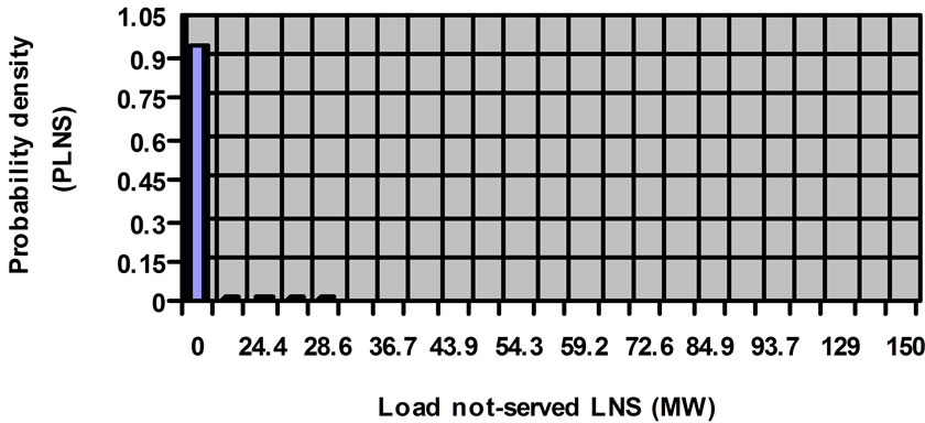
Using the results of the probabilistic analysis of Hail system, the discrete probability density functions of various reliability and performance quality indices can be evaluated and displayed. These discrete density functions show the overall probabilities of occurrence associated with certain values of the system performance indices. The probability density function of the Load Not Served (LNS) for Hail network at required load level 150 MW is depicted in Figure 6(a). Also, Figure 6(b) shows the probability density of the Surplus Generation Capacity (Qg011) at load level 200 MW.
Some valuable information can be drawn from the probability density functions of Figures 6(a) and (b). For example, the probability of Load Not Served (LNS) in Hail being zero when the required load level is 150 MW is 0.9387
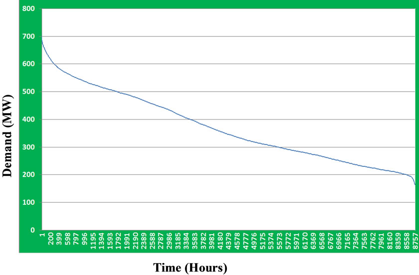
Figure 5. Hail load duration curve.
 (a)
(a)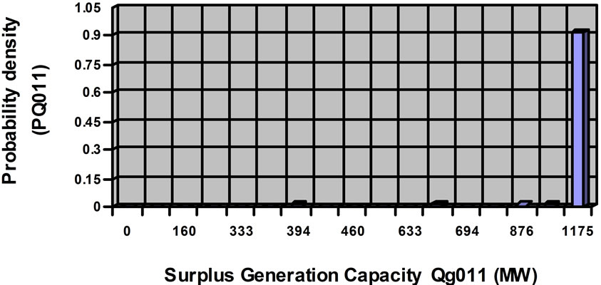 (b)
(b)
Figure 6. (a) Probability density of load not served (LNS) for Hail network at load 150 MW; (b) Probability density of surplus generation capacity (Qg011) for Hail network at load 200 MW.
(from Figure 6(a)) while there is a probability of 0.0310 that the unsupplied load is equal to, or greater than 25 MW. On the other hand, there is a probability of 0.92 that the Surplus Generation Capacity (Qg011) in Hail (at load level 200 MW) is equal to, or greater than 1175 MW.
When all required load levels are considered with their respective probabilities of occurrence (as per the load duration curve), an overall estimate of the expected value of reliability and performance quality indices can be obtained as shown in Table 2.
The overall expected value of the Load Not Served (LNS) for Hail is 4.01 MW, which is less than 1% of the required load in Hail. On the other hand, overall expected value of the Bottled Generation Capacity (Qg110) is 3.86 (MW),
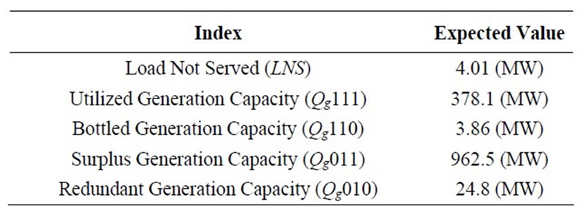
Table 2. Expedited values of reliability and performance quality indices for Hail network.
which again is less than 1% of the total Hail generation. It is also of interest to note that the overall expected value of the Utilized Generation Capacity (Qg111) is 378.1 (MW), which represents almost 64% of the total generation capacity in Hail. In other words, about 36% of Hail available generation capacity is expected to be unutilized. Recalling from Table 1 that the Hail generation capacity is 594 MW (base value) while the required base load is 655 MW, one may conclude that the 64% expected value for the utilized generation is a reflection of the relatively large variations of the required load during different periods of the year, as is evident from the load duration curve of Figure 5.
5. Conclusions
The work of this paper represents a major extension to the previously published work by developing a theory and formulas for computing the expected values of different system reliability and performance quality indices. The reliability and performance quality indices, when evaluated at a given load level and a certain scenario of available generation and transmission capacities, would provide indication on system performance for only such a particular system condition (snapshot). However, the novel formulation presented in this paper can accommodate the randomness associated with the load level as well as the availability of generation and transmission capacities. In this case, expected values of reliability indices, such as the Expected Load Not-Served (eLNS), as well as the expected values of performance quality indices, such as Utilized Generation Capacity (eQg111), Bottled Generation Capacity (eQg110), Shortfall Generation Capacity (eQg101), Deficit Generation Capacity (eQg100), Surplus Generation Capacity (eQg011), Redundant Generation Capacity (eQg010), Spared Generation Capacity (eQg001) and Saved Generation Capacity (eQg000) can be calculated using the load duration curve as well as the availability rates of generation and transmission facilities in the system.
The results of the probabilistic analysis of Hail system have revealed that the probability of Load Not Served (LNS) in Hail being zero (when the required load level is 150 MW) is 0.9387, while there is a probability of 0.0310 that the unsupplied load is equal to, or greater than 25 MW. When all required load levels are considered with their respective probabilities of occurrence (as per the load duration curve), an overall estimate of the expected value of reliability and performance quality indices were obtained for Hail where the overall expected value of the Load Not Served (LNS) is 4.01 MW, which is less than 1% of the required load in Hail. On the other hand, overall expected value of the Bottled Generation Capacity (Qg110) is 3.86 (MW), which again is less than 1% of the total Hail generation.
6. Acknowledgements
This work was supported by the Saudi Electricity Company.
REFERENCES
- H. Jun, Y. Zhao, P. Lindsay and P. Kit, “Flexible Transmission Expansion Planning with Uncertainties in an Electricity Market,” IEEE Transactions on Power Systems, Vol. 24, No. 1, 2009, pp. 479-488. doi:10.1109/TPWRS.2008.2008681
- M. El‑Kady, M. El‑Sobki and N. Sinha, “Reliability Evaluation for Optimally Operated Large Electric Power Systems,” IEEE Transactions on Reliability, Vol. R35, No. 1, 1986, pp. 41‑47. doi:10.1109/TR.1986.4335340
- M. El‑Kady, M. El‑Sobki and N. Sinha, “Loss of Load Probability Evaluation Based on Real Time Emergency Dispatch,” Canadian Electrical Engineering Journal, Vol. 10, 1985, pp. 57‑61.
- M. A. El-Kady and B. M. Alshammary, “A Practical Framework for Reliability and Quality Assessment of Power Systems,” Journal of Energy and Power Engineering (EPE), Vol. 3, No. 4, 2011, pp. 499-507. doi:10.4236/epe.2011.34060
- P. Jirutitijaroen and C. Singh, “Reliability Constrained Multi-Area Adequacy Planning Using Stochastic Programming With Sample-Average Approximations,” IEEE Transactions on Power Systems, Vol. 23, No. 2, 2008, pp. 405-513. doi:10.1109/TPWRS.2008.919422
- R. Billinton and D. Huang, “Effects of Load Forecast Uncertainty on Bulk Electric System Reliability Evaluation,” IEEE Transactions on Power Systems, Vol. 23, No. 2, 2008, pp. 418-425. doi:10.1109/TPWRS.2008.920078
- M. El-Kady, B. Alaskar, A. Shaalan and B. Al-Shammri, “Composite Reliability and Quality Assessment of Interconnected Power Systems,” International Journal for Computation and Mathematic in Electrical and Electronic Engineering (COMPEL), Vol. 26, No. 1, 2007.
- P. Gill, W. Murray and M. Wright, “Practical Optimization,” Academic Press, Waltham, 1981.