Communications and Network
Vol. 4 No. 2 (2012) , Article ID: 19106 , 26 pages DOI:10.4236/cn.2012.42021
Homogeneous and Heterogeneous Traffic of Data Packets on Complex Networks: The Traffic Congestion Phenomenon*
1SELEX Sistemi Integrati s.p.a., Roma, Italy
2CERI, Università di Roma “La Sapienza”, Roma, Italy
3Dipartimento di Scienze Sociali, Università Politecnica delle Marche, Ancona, Italy
Email: {afarina, agraziano}@selex-si.com, fra_mariani@libero.it, f.zirilli@caspur.it, m.c.recchioni@univpm.it
Received February 24, 2012; revised March 25, 2012; accepted April 15, 2012
Keywords: Complex Networks; Network Topology; Congestion Phenomenon; Small World Property; Phase Transition
ABSTRACT
We study the congestion phenomenon in a mathematical model of the data packets traffic in transmission networks as a function of the topology and of the load of the network. Two types of traffic are considered: homogeneous and heterogeneous traffic. The congestion phenomenon is studied in stationary conditions through the behaviour of two quantities: the mean travel time of a packet and the mean number of packets that have not reached their destination and are traveling in the network. We define a transformation that maps a network having the small world property (Inet 3037 in our numerical experiments) into a (modified) lattice network that has the same number of nodes. This map changes the capacity of the branches of the graphs representing the networks and can be regarded as an “interpolation” between the two classes of networks. Using this transformation we compare the behaviour of Inet 3037 to the behaviour of a modified rectangular lattice and we study the behaviour of the interpolating networks. This study suggests how to change the network topology and the branch capacities in order to alleviate the congestion phenomenon. In the website: http://www.ceri.uniroma1.it/ceri/zirilli/w6 some auxiliary material including animations and stereographic scenes that helps the understanding of this paper is shown.
1. Introduction
In this paper we study the data packet traffic congestion phenomenon in transmission networks in the case of homogeneous and heterogeneous traffic. This is an interesting phenomenon with several practical applications among which we mention the study of the behaviour of telecommunication networks and in particular of the behaviour of Internet. More in general the congestion problem in network flows is of great interest in several engineering fields, such as, for example, pipeline flow, electric power transmission [1], telecommunications and high-ways or railways traffic management. To fix the ideas let us consider the Internet traffic. The Internet network grows in size every day and its possible congestion is a relevant issue from the social and the economic point of view. In fact it is easy to image the damage that the Internet congestion will cause to the social relations and to the economic transactions that take place on it. In the last years several end-hosts have been added to the edge of the Internet network and these new entries have increased substantially the load of the network. The Internet Service Providers have added new routers and links to avoid the congestion arising from these new entries. Several authors have developed transmission network models devoting special attention to the network congestion problem (see for example [2] and the reference therein). Remarkable network models relevant in the study of Internet are those due to Aiello, Chung and Lu [3] that are based on power law random graph models, to Fabrikant, Koutsoupias and Papadimitriou [4] that propose a bicriteria optimization model and to Barabasi and Albert [5] that have introduced the preferential connectivity model. These models have a common feature: a power law distribution of the degree of the network nodes. Furthermore more practical models of the Internet network are those based on inferences drawn from measurements of real Internet data. In particular a huge effort has been produced to construct generators of graphs that reproduce the features actually measured in the Internet network (see for example [6,7]). Previous work that addresses the congestion problem in flow problems on graphs and more specifically the problem of designing routing schemes able to avoid congestion is, for example, the work contained in the papers of Aumann and Rabani [8], Okamura and Seymour [9], Leighton [10] and Leonardi [11]. In [8] and [9] the network congestion problem is formulated as a problem concerning the max-cut ratio of a graph while in [10] and [11] the problem of finding fractional routing strategies with good congestion properties is addressed. The data packet traffic is described by the routing strategy and by the traffic management rules. The routing strategy considered here to move the packets from their origin to their destination is the shortest weighted path. The traffic management rules are the rules used to manage the data packet traffic at the nodes where more than one data packet is waiting to be directed. The traffic management rules considered in our study are a simple variation of the “first in first out” rule.
Going into details let n be a positive integer, we model the transmission network using an undirected (weighted) graph G having n nodes. The graph G consists in the couple (V, E), where V is the set of nodes/vertices and E is the set of branches/edges/lines of the graph. The vertices are numbered, that is for a graph with n vertices we can choose V = {1, 2,…, n}. A branch is indexed by a couple of integers m, k ∈ V with m ≠ k, the branch em,k ∈ E connects the nodes m (source node) and k (destination node). For m, k ∈ V such that m ≠ k, if em,k ∈ E then ek,m ∈ E and ek,m denotes the same branch than em,k. Moreover, for em,k ∈ E we associate to the branch em,k a capacity cm,k > 0 and we denote with pm,k the inverse of cm,k, pm,k is the weight associated to the branch em,k. For em,k ∈ E the capacity cm,k is a positive integer and is the maximum number of data packets that can go through the branch em,k in a time unit moving from the source node m to the destination node k. Moreover for em,k ∈ E we assume that cm,k = ck,m and as a consequence that pm,k = pk,m. We extrapolate this relation and we say that when the weight of a “branch” em,k is infinity its capacity is zero and this corresponds to the fact that no packet can flow through it. That is, given a couple of (distinct) nodes we can always imagine that there is a branch with zero capacity that connects them. We consider connected graphs, that is graphs G such that for every couple of (distinct) nodes (m, k) there exists a path made of branches (with capacity greater than zero) connecting the source node m to the destination node k. The degree of a node is the number of branches (with capacity greater than zero) that have the node as source node (or as destination node). In the generation of the data packet traffic the source and the destination nodes of the data packets are sampled from a random variable uniformly distributed on the set of the couples of (distinct) nodes of the graph. A data packet can move from a node to another node in one time unit if there is a branch (with capacity greater than zero) that connects the two nodes, that is, if the nodes are adjacent nodes in the graph. The movement of a data packet from a node to one of its adjacent nodes is always made in one time unit. To each couple of distinct nodes (m, k) (source, destination), m, k = 1, 2, ∙∙∙, n, we associate a route that is the path that a data packet moving from m to k must follow, this route is the shortest weighted path connecting m to k with some extra specifications explained later. The data packet travel time (or delivery time) is the time that elapses between the creation of the packet at its source node m and the arrival of the packet at its destination node k. The travel time is measured in time units. Each node is equipped with queues, which is in each node there is a queue for each branch (with capacity greater than zero) leaving the node. When a branch departing from a node is busy (i.e. its capacity is saturated) a packet arriving or already present at that node directed through that branch toward its destination is put in the node queue relative to that branch and waits the successive time units to be directed. The node queues are assumed to be potentially unbounded and, of course, eventually, they can be empty. The management of the queues is done through the traffic management rules. In the case of homogeneous traffic, that is when only one kind of data packets is moving on the network, the queue management rule is simply based on the arrival order of the packets at the node, which is the traffic management rules consist in only one rule: the first in first out rule with the following specifications added. Let us restrict our attention to the packets present at a node that are leaving the node (following their routes) through a given branch. Note that when two or more packets must go through the same branch and this branch has sufficient capacity available the packets go through the branch simultaneously, that is, they go through the branch in the same time unit. When two or more packets must go through the same branch and there is no sufficient capacity available on the branch to let them go simultaneously we use the “first in first out” rule, that is we deliver first the packet that arrived first at the node. When two or more packets that must go through the same branch are the “first arrived one” at the node we deliver first the packet that has been generated earlier. Note that the packet that is delivered first is the one that goes first in the queue. When two or more of these first arrived packets that have been generated earlier have been generated at the same time we choose randomly between these last packets the packet to move first. In the study of the heterogeneous traffic case we limit our attention to the case that there are three kinds of data packets moving on the network. The choice of studying as heterogeneous traffic case the traffic of three kinds of data packets is inspired by the fact that in real telecommunication networks we can distinguish data, video and voice packets. In this last case the traffic management rules are specified as follows. We associate to each packet waiting at a busy node a waiting time measured in time units based on the arrival order at the node. For the packets of kind i we multiply this waiting time for the priority factor pi of the kind i packets, i = 1, 2, 3. The priority factors are chosen as follows: p1 = 3 for the packets having highest priority (packets of kind i = 1), p2 = 2 for the packets having intermediate priority (packets of kind i = 2) and p3 = 1 for the packets having lowest priority (packets of kind i = 3). The queue management rule consists in the choice of moving first the packet having the largest product waiting time at the node times priority factor. When two or more packets have the largest product waiting time at the node times priority factor we deliver first the packet that has been generated earlier. If at a node two or more packets having the largest waiting time times priority factor that have been generated earlier have been generated at the same time we choose randomly between these last packets the packet to move first. Of course also in the case of heterogenous traffic when there is capacity available more than one packet can go through the same branch at the same time. Note that the heterogenous traffic case reduces to the homogeneous traffic case when we choose p1 = p2 = p3. For simplicity we present the load model used later directly in the heterogeneous traffic case. We leave to the reader to find out the simple changes necessary to describe the load model in the homogeneous traffic case. We model the number of kind i packets, Mi, generated in the network in a time unit as a Poisson random variable with mean βiλ, i = 1, 2, 3, where βj, j = 1, 2, 3, are given nonnegative constants such that  and λ > 0 is a real parameter. The choice of the constants βj, j = 1, 2, 3, determines different heterogeneous load conditions on the network. Later we consider three choices of the constants βj, j = 1, 2, 3. The first one is β1 = β2 = β3 = 1/3, that generates a balanced load condition, that is generates a load having in average the same number of packets for the three kinds of packets. The second one is β1 = 5/7, β2 = 1/7, β3 = 1/7, that generates an unbalanced load condition, that is generates a load having in average a large number of packets with highest priority (kind i = 1) and such that the remaining two kinds of packets have (in average) a smaller number of packets, in particular since β2 = β3 they have (in average) the same number of packets. The last one is β1 = 1/6, β2 = 2/6, β3 = 3/6, that generates the most common load situation in real networks, that is the situation where the number of packets with the highest priority (kind i = 1) is (in average) smaller than the number of packets with intermediate priority (kind i = 2) and this last number is (in average) smaller than the number of packets with lowest priority (kind i = 3).
We call congestion phenomenon for the (kind i) data packet traffic the passage from a free flow to a congested flow (i = 1, 2, 3). We study the congestion phenomenon in stationary conditions using the following two quantities: the mean travel time of kind i data packets,  , and the mean number of kind i packets that have not reached their destination and are travelling on the network,
  , i = 1, 2, 3. Our analysis shows that, in the free traffic regime and in stationary conditions, for i = 1, 2, 3 the quantities
  and
and  are independent of time and that they increase when the network mean loads βjλ, j = 1, 2, 3, increase. Given the weighted graph G, and the constants βj, j = 1, 23, such that βj ≥ 0, j = 1, 2, 3, and
 , for i = 1, 2, 3 we study the quantities
  and
and  as a function of the parameter λ. We will see from the numerical simulations that some expressions specified later involving
  and
and  have a jump for a value of the parameter λ that we denote with λ =
 , i = 1, 2, 3. For the traffic of kind i packets the value λ =
  represents the so called critical value of the parameter λ that divides the zone of congested traffic (βiλ > βi
 ) from the zone of free traffic (βiλ < βi
 ), i = 1, 2, 3. Note that strictly speaking when λ >
  the quantities
  and
and  do not have a stationary value in time anymore, in fact in this case these quantities diverge when time increases, i = 1, 2, 3. Under specified traffic conditions we have evaluated through extensive simulations these critical values λ =
 , i = 1, 2, 3, as a function of the network topology.
Our analysis shows that the networks having the small world property (see, for example, the network of Figure 1) and the (possibly modified) lattice networks, that do not have the small world property, (see, for example, the network of Figure 3) behave very differently with respect to the congestion phenomenon. In particular we have compared the behaviour of Inet 3037 (Figure 1) to the behaviour of a modified rectangular network (Figure 3) made of a rectangular lattice having 3036 nodes and of an extra node of degree four. Note that Inet 3037 is a network made of 3037 nodes generated using the software package [6] (algorithm Inet-3.0) that is supposed to reproduce the properties of the AS-level Internet graph topology. The empirical analysis of the AS-level Internet graph topology goes back to 1999 with the work of M. Faloutsos, P. Faloutsos, C. Faloutsos [12] that has shown that the Internet node degree distribution decays as a power-law, that is the function F'(k) = {percentage of the nodes with degree greater or equal to k} associated to AS-level Internet
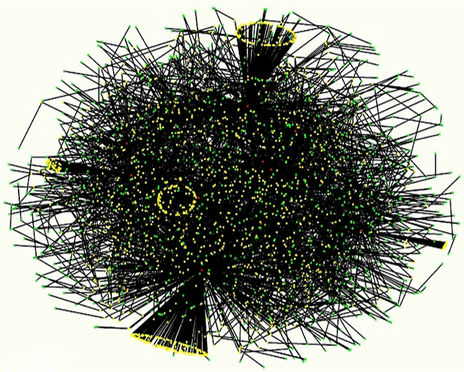
Figure 1. Inet 3037.
graphs behaves like k−β, with β = 2.22, for large values of k (see Section 2 formula (1)). This property is usually stated saying that Internet at the AS-level graph is a scale free network. Later in 2002 Subramanian, Agarwal, Rexford, Katz [13] have shown that a realistic model of the ASlevel Internet graph topology is a “power law topology” with a core structure. This core structure is a subset of nodes having large degree that is called rich-club (see, for example, Figure 2 where the rich club of Inet 3037 is shown). The nodes belonging to the rich club are well connected between themselves by paths of short length (and high capacity), moreover they are connected to the remaining nodes by paths of short length. We recall that a network having this feature is said to have the small world property. When routing strategies such as the shortest path or the shortest weighted path are used to deliver the packets the rich club is similar to a set of traffic hubs. The network model due to Barabasi and Albert [5] and the Inet- 3.0 algorithm [6] used to generate graphs with AS-level Internet graph topology consider scale free networks with β ∈ (2, 3), however in these models the reproduction of the Internet core structure is not completely satisfactory. In fact in these models the rather sophisticated structure of the rich club observed in the real Internet is replaced with just a few nodes having very large degree, and these nodes play the role of network hubs in the study of data packets traffic.
We consider, for a moment, networks where all the branches have the same capacity and the shortest path routing strategy. In the free traffic region we show that a network having the small world property is much more efficient in the delivering of packets in terms of travel time than a lattice network of similar “size”. However when the load increases a network having the small world property and the same capacity on all its branches reaches the congested regime for smaller values of the load than a lattice network of similar “size”. When we consider net-
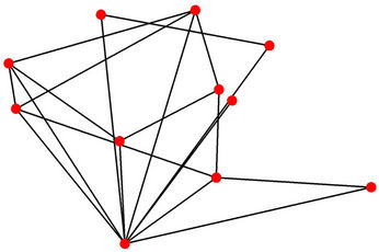
Figure 2. The rich club of Inet 3037.
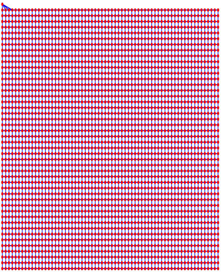
Figure 3. The modified rectangular lattice.
works where the branches do not have necessarily the same capacity and the capacities are chosen in order to exploit the small world property this phenomenon occurs in a more subtle way. We investigate this phenomenon studying Inet 3037 (see Figure 1) in comparison to a modified rectangular lattice network (see Figure 3). Note that these two networks have the same number of nodes. This fact motivates the idea of defining a transformation, depending on a parameter α ∈ [0, 1], that maps the network having the small world property Inet 3037 (i.e.: α = 0) into the modified rectangular lattice network (i.e.: α = 1). This transformation acts changing the weights of the branches of the networks and depends on the way the nodes of the networks are numbered. Note that in this paper the node numbering is given and that the dependence of the transformation between networks mentioned above and of the phenomena studied on the networks from the numbering of the nodes is not considered. Given the constants βj, j = 1, 2, 3, we study the critical values of the parameter λ = , i = 1, 2, 3, as a function of the parameter α and of the traffic management rules. This study suggests some changes in the traffic management rules and/ or in the network topology able to alleviate the consequences of the congestion phenomenon. Some analogies between the congestion phenomenon studied here and the phase transition phenomenon studied in statistical mechanics are illustrated. In the web site:
http://www.ceri.uniroma1.it/ceri/zirilli/w6 some auxiliary material including animations and stereographic scenes that helps the understanding of this paper is shown.
The paper is organized as follows. In Section 2 we describe the topological properties of Inet 3037 and of the modified rectangular lattice network. Using the fact that Inet 3037 and the modified rectangular lattice network considered have the same number of nodes we define a transformation depending on a parameter α ∈ [0, 1] that maps Inet 3037 (i.e. α = 0) into the modified rectangular lattice network (i.e. α = 1). In Section 3 in the homogeneous traffic case we study the traffic congestion phenomenon on Inet 3037, on the modified rectangular lattice network considered in Section 2 and on the α- networks, α ∈ (0, 1). In Section 4 in the heterogeneous traffic case we study the traffic congestion phenomenon on the previous networks. Finally in Section 5 we draw some conclusion.
2. The Networks and Their Topological Properties
The topological features of a graph that will be considered in our analysis are: the node degree distribution, the mean length of the shortest path between the couples of (distinct) nodes, the betweenness centrality of the nodes and the graph connectivity. These purely topological notions are adapted to the fact that the networks considered are modeled as weighted graphs, that is are adapted to the fact that we have capacities associated to the branches of the graphs.
Let G = (V, E) be a graph having n nodes that models a network. For k = 0, 1, ∙∙∙, n−1, let f(k) be the frequency of the nodes of the graph having degree k, and let F(d), d = 0, 1, ∙∙∙, n−1, be the node degree cumulate distribution, that is
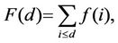 d = 0, 1, ∙∙∙, n−1, we define F′(d) = 1−F(d), d = 0, 1, ∙∙∙, n−1. We say that a network is a scale free network when the function F′(d) decays as an inverse power of d when d increases (see Figure 4), that is when we have:
 (1)
(1)
for some positive constants c and β (see [6]).
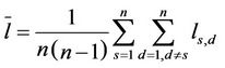
The mean length of the shortest path is the mean value
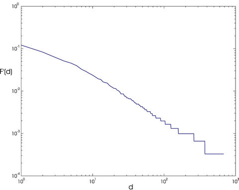
Figure 4. F′(d) as a function of the node degree d.
 (2)
(2)
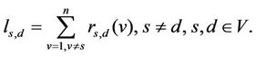
of the length of the shortest path that joins the couples of (distinct) nodes, (s, d), s ≠ d, s, d ∈ V, that is: where ls,d is the length of the shortest path connecting the nodes s and d, s ≠ d, s, d ∈ V, that is ls,d is the smallest number of nodes that must be visited to go from s to d, s ≠ d, moving on branches with capacity greater than zero, s, d ∈ V. Note that when evaluating the length of a path that goes from s to d the node d must be counted between the nodes visited to go from s to d. We consider connected graphs so that for every couple of nodes (s, d), s ≠ d, s, d ∈ V there is at least one path that goes from s to d. Note that the shortest path between two nodes may be nonunique. In our analysis we consider weighted graphs and as a consequence weighted paths so that we consider the mean length of the shortest weighted path defined as the mean value of the length of the shortest weighted path that joins the couples of network nodes. That is, let Ss,d be the set of the paths connecting the nodes s and d, s ≠ d, s, d ∈ V. The shortest weighted path between the nodes s and d, s ≠ d is the path  ∈ Ss,d that goes from s to d having the smallest sum of the inverse of the capacities of its branches, s, d ∈ V. Note that the shortest weighted path may be nonunique. When it is nonunique we choose as
 ∈ Ss,d that is, as the shortest weighted path whose length is used in (5), the path that is determined by the algorithm used to compute it. Let
  be defined as follows:
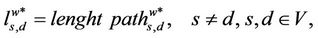 (3)
(3)
where with the previous specifications we define:
 (4)
(4)
The mean length of the shortest weighted path of the graph G can be defined as follows:
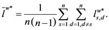 (5)
(5)
Note that  is not well defined when the shortest weighted path is not unique, that is the definition given above is loose. In fact different shortest weighted paths may have different lengths and different algorithms to determine them may determine different paths. More satisfactory definitions can be given at the price of making the exposition more complicated. These definitions will be omitted. Remind that when we consider Inet 3037 for every branch em,k ∈ E the weight pm,k of the branch is a positive number equal to the inverse of the capacity cm,k of the branch that is assigned by the Inet-3.0 algorithm [6].
The betweenness centrality of a node v ∈ V is the following quantity:
 (6)
(6)
where rs,d(v), s ≠ d, s ≠ v, d ≠ v, is the number of the shortest paths joining s to d passing through the node v divided by the total number of the shortest paths joining the node s to the node d, s, d, v ∈ V. Note that we have:
 (7)
(7)
We generalize the betweenness centrality defined in (7) introducing the weighted betweenness centrality of a node v ∈ V defined as follows:
 (8)
(8)
where , s ≠ d, s ≠ v, d ≠ v, is the number of the shortest weighted paths joining s to d passing through the node v divided by the total number of the shortest weighted paths joining the node s to the node d, s, d, v ∈ V. The weighted betweenness centrality adapts the notion of betweenness centrality to the fact that we consider weighted graphs. Note that the betweenness centrality and the weighted betweenness centrality of a node are measures of the “relevance” of the node for the traffic on the network when we use as routing strategy respectively the shortest path and the shortest weighted path. Roughly speaking they are measures of how much a node acts as a hub in the network when we use the routing strategies mentioned above.
Let us consider a graph G = (V, E) and the nonempty sets S ⊆ V such that the graph G\S = (V\S, E ∩ ((V\S) × (V\S))) is a disconnected graph and the set Σ of the cardinalities of the sets S that have the previous property. The connectivity of the graph G is the minimum of the set Σ. Roughly speaking the connectivity of a graph is the smallest number of nodes that must be removed from the graph to disconnect it.
Let us describe the Inet 3037 network. The Inet 3037 network has been generated using the package Inet (Internet Topology Generator) (see [6] for further details). The algorithm used by the Inet package is the Inet-3.0 algorithm and generates random graphs modeling the ASlevel Internet graph topology. In fact Internet can be viewed as an AS-level topology graph where each AS (Autonomous Systems) is a node, and the BGP (Border Gateway Protocol) peering between two ASes is a link. Inet-3.0 takes into account the Internet topological properties as observed by the University of Michigan research team that has implemented and distributes the Inet package. For example, it considers the node degree distribution and the network connectivity of the graphs generated. In detail, the Inet-3.0 algorithm takes as input the number n of nodes that the network generated must have and the number of nodes of the network that must have degree one. Taken these two input data Inet-3.0 generates a graph whose links are chosen in order to reproduce the result of a study of the node degree distribution, of the connectivity and of some other properties of Internet as registered in the BGP (Border Gateway Protocol) routing tables of the Oregon server: route-views.oregon-ix.net. The Oregon server collects information on the traffic over autonomous systems belonging to distinct Internet service providers and on their topology communicating with these providers through the BGP protocol. The output of the Inet-3.0 algorithm are the links of the graph generated and a set of positive integers associated to the links that we interpret as capacities of the links. We have used Inet-3.0 to generate a weighted graph with n = 3037 nodes and we have required that approximately 30% of the nodes of the graph generated (to be precise 911 nodes) must have degree one. The connectivity of the graph generated by Inet-3.0 is 3, that is the integer part of 0.001·n. The resulting graph is Inet 3037 (see Figure 1). We note that in Inet 3037 the mean value of the node degree is approximately 3 and that the maximum value of the node degree is 684. The nodes having degree greater than 60 are 11 and are the red nodes shown in Figures 1 and 2. These nodes are the nodes of the rich club of Inet 3037. Figure 2 shows the nodes of the rich club of Inet 3037 and the branches of Inet 3037 that connect them. The red nodes appearing in Figures 1 and 2 can be considered as representatives of suitably defined subgraphs. A node y of Inet 3037 (a yellow node in Figure 1) belongs to a subgraph whose representative node is a node k of the rich club (red node in Figure 1) if there exists at least one path (made of branches with capacity greater than zero) joining y to k and there are no paths joining y to a node of the rich club different from k that do not go through k. The nodes such that there are paths joining them “directly” to more than one node of the rich club are represented as green nodes in Figure 1. The nodes of Inet 3037 are numbered in increasing order for decreasing values of the node degree. The nodes that have the same degree are numbered randomly with consecutive numbers. Inet 3037 has 4788 branches. The smallest and largest capacities of the branches are 67 and 12441 respectively. The mean value of the capacities of the branches of Inet 3037 is approximately 5064. An easy computation shows that Inet 3037 has ≈ 5.1649. Let us denote with RI(v) the sum of the capacities of the branches of Inet 3037 arriving at (or departing from) the node v, v ∈ V. Figure 5 shows the quantity RI(v) as a function of v ∈ V. We note that the first eleven nodes (i.e. the nodes numbered from one to eleven that are the nodes of the rich club) are those with highest degrees and with the highest values of RI.
Let us describe the modified rectangular lattice network that we use as a comparison term in the study of the behaviour of Inet 3037. The modified rectangular lattice network (see Figure 3) has 3037 nodes and is characterized by the degree of the inner nodes that is equal to four and by the capacity of its branches that is the same for all branches. The modified rectangular lattice network shown in Figure 3 has 5964 branches. The capacity of its branches, cR, is chosen as the integer part of the sum of the capacities of the branches of Inet 3037 divided by the number of branches of the modified rectangular lattice network. An easy computation gives cR = 4066. Note that since all the branches of the modified rectangular lattice have the same capacity the choice of cR made guarantees that the total capacity installed on Inet 3037 and the total capacity installed on the modified rectangular lattice network are roughly the same. They are roughly the same and not exactly the same since we have used the integer part to define the branch capacity of the modified rec-
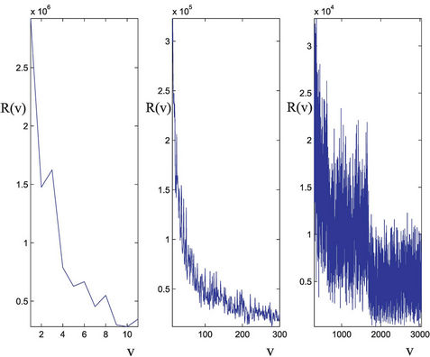
Figure 5. RI(v) as a function of the node number v.
tangular lattice. The use of the integer part in the definition of the branch capacity is due to the fact that the capacities are supposed to be integer numbers. In a m × l rectangular lattice network the inner nodes have the same betweenness centrality and the mean length of the shortest path is given by:
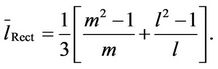 (9)
(9)
To build the modified rectangular lattice network we consider a m × l rectangular lattice network with m = 46 and l = 66, that is a network with 3036 nodes, and we add to it an extra node having degree four (see Figure 3). The nodes of the m × l rectangular lattice are numbered from right to left, and from the bottom row to the first row (see Figure 3) in increasing order beginning with v = 1 corresponding to the right bottom corner of the network. In particular let AR = ((ARi,j)) ∈ R3037×3037 be the weighted adjacency matrix of the modified rectangular lattice network defined starting from the weighted adjacency matrix of the 46 × 66 rectangular lattice network (with all the branches of capacity cR) adding to it an extra node, v = 3037, connected to the rectangular lattice network as shown in Figure 3, that is adding an extra row and column to the adjacency matrix of the 46 × 66 rectangular lattice as follows:
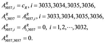 (10)
(10)
It is easy to see that the network modeled by the graph corresponding to the adjacency matrix AR is the one shown in Figure 3. The length of the mean shortest path in the modified rectangular lattice network shown in Figure 3 is ≈ 38.3424 ≈
 . Let us define the weights of the branches of the modified rectangular lattice network as the inverse of their capacities and let
  be the mean length of the shortest weighted path of the modified rectangular lattice, we note that since all the branches of the modified rectangular lattice network have the same capacities, they have also the same weights so that we have
 .
.
In the numerical simulations we scale the capacities of the branches of Inet 3037 and of the modified rectangular lattice by dividing them by the smallest capacity of the branches of Inet 3037 that is dividing them by 67. This choice reduces the computational work needed to carry out the numerical simulations.
Note that Table 1 shows that the nodes of the modified rectangular lattice have approximately the same relevance in terms of betweenness centrality, in fact for the modified rectangular lattice the mean value of the betweenness centrality is of the same order of magnitude of its maxi-

Table 1. Some features of Inet 3037 and of the modified rectangular lattice.
mum value. This is a consequence of the fact that the modified rectangular lattice does not have the small world property. The case of Inet 3037 is substantially different, in fact for Inet 3037 the mean value of the betweenness centrality is three orders of magnitude smaller than its maximum value.
Roughly speaking, in the case of Inet 3037, the node where the betweenness centrality reaches its maximum value (i.e. the node v = 1) absorbs approximately 58% of the traffic when we use the shortest path routing, that is about 58% of the shortest paths goes through this node. This percentage reduces to 46% if we consider the weighted shortest path routing and as a consequence the weighted betweenness centrality instead than the betweenness centrality.
Finally, for Inet 3037 we note that the sum of the betweenness centrality of the nodes of the rich club is 52% of the sum of the betweenness centrality of all the nodes and that the sum of the capacities of the branches connected to the nodes of the rich club is 41% of the sum of the capacities of all the branches of the network. In the case of the modified rectangular lattice (when we consider as rich club of the modified rectangular lattice the graph associated to its first eleven nodes, that is the nodes numbered from 1 to 11) the same ratios are approximately equal to 0.003% and to 0.03% respectively. Note that the correspondence between the rich club of Inet 3037 and the graph associated to the first eleven nodes of the modified rectangular lattice is a rather arbitrary one. In fact when we consider the modified rectangular lattice there is no a natural candidate to play the role of the rich club. Table 1 summarizes the topological properties of Inet 3037 and of the modified rectangular lattice discussed above.
Let EI denote the set of branches of Inet 3037 and AI ∈ R3037×3037 denote the weighted adjacency matrix of Inet 3037, that is the matrix whose entries are: , i ≠ j and
 , where
  if ei,j ∈ EI or
  if ei,j ∉ EI, i, j = 1, 2, ∙∙∙, 3037. Let α ∈ [0,1] be a real parameter, we denote with Aα = ((
 )) ∈ R3037×3037 the following combination of the weighted adjacency matrices AR and AI relative to the modified rectangular lattice and to Inet 3037 respectively:
 (11)
(11)
where  is the ceiling part of · and the ceiling part of a matrix is defined as the matrix whose entries are the ceiling parts of the entries of the original matrix. Remember that the ceiling part of a real number x is the smallest integer greater or equal to x. The matrix Aα is the weighted adjacency matrix of a graph that we call α-network, α ∈ [0, 1]. Note that when α = 0 we have Aα equal to the weighted adjacency matrix of Inet 3037 and when α = 1 we have Aα equal to the weighted adjacency matrix of the modified rectangular lattice. We note that in the transformation (11) the most important hub of Inet 3037, that is the node v = 1, is mapped into the node v = 1 of the modified rectangular lattice (that is, it is mapped in the bottom right corner of the modified rectangular lattice, see Figure 3) and so on. This correspondence between the nodes is somehow arbitrary and depends on the way the nodes are numbered.
Note that since the mean shortest weighted path of the modified lattice network is about seven times greater than the mean length of the shortest weighted path of Inet 3037 in the numerical simulation of the traffic flow (in the free flow regime) on these networks we expect that a similar relationship holds between the simulation times needed to reach the stationary condition. We can conclude that the time interval simulated must be chosen appropriately in order to guarantee that on both networks the stationary regime has been reached.
Let us make some comments about the topological features of the α-networks. Let us denote with GI = (VI, EI), GR = (VR, ER) and Gα = (Vα, Eα), α ∈ [0, 1], the graphs associated respectively to Inet 3037, to the modified rectangular lattice and to the α-network, α ∈ [0, 1]. We have VI = VR = Vα, α ∈ [0, 1], and EI = E0, ER = E1, moreover for any α ∈ (0, 1) we have Eα = EI ∪ ER, α ∈ (0, 1). This implies that for α ∈ (0, 1) the mean length of the shortest path of the α-network  is smaller or equal than
  and
and .
.
Table 2 shows that, at least for the values of α considered in Table 2, this property continues to hold when we consider the shortest weighted path. This is not obvious and depends on the weights associated to the branches. Note that between the α-networks considered in Table 2 the one having the smallest mean length of the shortest weighted path is the α = 0.5-network.
The capacities of the branches of the α-network are
 , ei,j ∈ Eα and the corresponding weights used in (4) are
 , ei,j ∈ Eα, α ∈ [0, 1].
Note that when α goes from zero to one in (11) in the α- network we have a reduction of the capacities of the
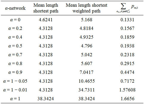
Table 2. Some features of the α network.
branches connected to the hubs of Inet 3037 and that this implies the reduction of the weighted betweenness centrality of the hubs. This fact makes possible to reduce the mean length of the shortest path since the advantage of going through the hubs in the shortest weighted paths (see [14]) is reduced.
Finally, let α ∈ [0, 1] for the graph Gα consider the weighted betweenness centrality , v ∈ Vα defined as in (8). For several choices of α, such that α ∈ [0, 1], Table 4 shows the corresponding values of the maximum,
  , with respect to v of
 , v ∈ Vα.
3. The Traffic Congestion Phenomenon in the Homogeneous Traffic Case
Let us study the congestion phenomenon in the homogeneous traffic case for the networks described by the weighted adjacency matrices defined in (11). Note that the homogeneous traffic case can be obtained as a special case of the heterogeneous traffic case, for example, with the choice of the priority factors: p1 = p2 = p3 = 1 or with the choice β1 = 1, β2 = β3 = 0. Then in the homogeneous traffic case the mean load of packets generation is equal to β1λ = λ. At time zero the networks studied are empty, that is they do not contain data packets. This fact generates a transient behaviour that connects the initial state (i.e. empty network) to the large time behaviour of the traffic on the network. For the homogeneous and the heterogeneous traffic case the simulation of the data packet traffic is carried out in the time interval [0, T]. The time T is chosen to be 400 time units in order to guarantee that in the free flow regime the traffic on the networks considered has (approximately) reached the stationary condition. The simulation procedure in the homogeneous traffic case consists of the following steps:
1) choose the number Nα + 1 of the network topologies that will be considered in the simulations, we consider Nα = 10;
2) choose the network topologies, that is, assign the values of α used in the simulations, we consider α = αj = (j−1)/Nα, j = 1, 2, ∙∙∙, Nα+1;
3) define the topology of the networks studied, for j = 1, 2, ∙∙∙, Nα+1, we consider the network associated to the weighted adjacency matrix  defined by (11) when α = αj, this is the α = αj-network topology;
4) packets generation: in each time unit of the simulation we first sample from a Poisson random variable with mean λ the number of packets generated in that time unit. The values of λ considered in the simulations are 201 values equispaced in the interval [10, 3000], that is we choose λ = λk = 10 + (3000−10)k/200, k = 0, 1, ∙∙∙, 200. A couple of nodes are assigned to each packet generated. This couple of nodes is sampled from a random variable uniformly distributed on the set of couples (s, d), such that s ≠ d, s, d = 1, 2, ∙∙∙, 3037. For s, d = 1, 2, ∙∙∙, 3037, s ≠ d, the packet associated to the couple (s, d), originates in the node s and its destination is the node d;
5) routing: the routing consists in associating to each packet a shortest weighted path connecting the node where the packet originates with its destination node. The packet is forwarded along this path during the time steps that follow the time of its generation. When the shortest weighted path between the origin and destination nodes of a packet is not unique the packet follows the shortest weighted path determined by the algorithm used to compute the routing of the packets (see [14]). When the packet reaches its destination is removed from the traffic simulation;
6) queue management: every node has a queue for each branch leaving the node, we assume the queues to be potentially unbounded. When a packet is generated in a node or arrives at a node, it is placed in the appropriate queue of the node in the process of being delivered toward its destination along its route. The queue management rule is: first in first out. When two or more packets that must continue their route on the same branch arrive simultaneously at a node the one that goes first in the queue is the packet that has been generated earlier. When two or more packets that must continue their route on the same branch and that have been generated simultaneously arrive simultaneously at a node we choose randomly between them the one that goes first in the queue;
7) packets movement: in a time unit, when there is capacity available on the relevant branch, a packet moves from the node where it is to the adjacent node along its route (i.e. the shortest weighted path). When there is no capacity available on the relevant branch the packet waits the next time unit at the node where it is. Remember that in each time unit, when in a node i we have several packets that (according with their routes) must be delivered to the same adjacent node j we deliver them in the same time unit as long as the number of packets delivered in the time unit on the branch ei,j is smaller or equal than the capacity of the branch ei,j. For example for the α-network the maximum number of packets that can be forwarded in the same time unit along the branch ei,j ∈ Eα is , α ∈ [0, 1]. This procedure applies to every node and to every branch.
We note that the parameter λ is the mean value of the number of packets generated in the entire network in a time unit, so that given the fact that the origin and the destination nodes attributed to the packets are sampled from an uniformly distributed random variable and the fact that there are n nodes in the network we can conclude that every node on average generates λ/n packets per time unit.
Note that we have chosen as routing strategy the shortest weighted path (see formula (3)) instead than the more usual shortest path. This choice is made in order to take advantage of the network complexity, that is of the small world property enjoyed by Inet 3037 (and by the α-networks, α ∈ (0, 1)), and of the fact that the branches of Inet 3037 have capacities ranging in a wide interval in a way that makes possible to take advantage of the small world property. In fact in the case of Inet 3037 the use of the shortest path route will direct almost all the packets through the nodes with higher betweenness centrality resulting in an inadequate exploitation of the branch capacities and ultimately in traffic congestion. Note that in the modified rectangular lattice case (i.e.: α = 1), due to the choice of giving the same capacity to all the branches, the shortest path and the shortest weighted path routing strategies coincide.
In the homogeneous traffic case let NL, tM be respectively the quantities analogous to the quantities , i = 1, 2, 3, introduced previously in the heterogenous traffic case. Note that in NL, tM we drop the subscript i, since in the homogeneous traffic case there is only one kind of data packets travelling on the network, that is we have only i = 1. The traffic simulation shows that, when there is no congestion, after a transient time, whose duration depends on the network topology, the traffic flow reaches a stationary state where, in average, the total number of packets created and delivered are equal, that is NL is a finite quantity and the mean travel time tM measured in time units is of the order of magnitude of the mean length of the shortest weighted path. This last fact is a natural consequence of Little’s law of queueing theory [15]. This stationary state is the free flow state. When λ increases we observe that the traffic on the network goes from the free flow state to a congested state and that this transition can be characterized by a value λ* of the parameter λ, that separates these two different states. The value λ* is called critical value of λ. Note that when λ is greater λ* there is no a stationary state (in time) for the traffic on the network, that is, the quantities NL and tM increase monotonically towards infinity when the simulation time goes to infinity.
Let us define the criteria that establish in the numerical simulation when a value of the load parameter λ is critical.
Let us denote with tα the mean length of the shortest weighted path expressed in time units. Moreover, since we want to put in evidence the dependence of the quantities NL and tM on the parameters α and λ let us use the notation  and
and , λ > 0, α∈ [0, 1]. Note that when the load parameter λ is below the critical value (that is the network traffic is after a transient period in the free flow state) we have
  ≈ tα and
 ≈ λtα.
In the numerical simulations we use two criteria to recognize the critical values of λ:
Criterion 1: Given an α-network we say that λ* is the critical value of the load parameter λ for the α-network when λ* is the smallest value of λ such that the derivative with respect to λ of  measured using λ as unit, that is the quantity
 , is greater than a given positive constant γ.
Criterion 2: Given an α-network we say that λ* is the critical value of the load parameter λ for the α-network when λ* is the smallest value of λ such that the derivative with respect to λ of the mean travel time measured using tα as unit, that is the quantity , is greater than a given positive constant γ.
The choice of the threshold γ depends on the network and on the criticality criterion considered.
Let us study the critical value of λ as a function of α, α ∈ [0, 1]. The numerical simulations show that going from Inet 3037 (α = 0) to the modified rectangular lattice (α = 1) the critical value of the parameter λ, λ = λ*(α), as a function of α has a maximizer for a value of α ∈ (0, 1). This maximizer depends on the value of γ. In particular, Figure 6 shows the critical values of λ as a function of α for four choices of the threshold γ, that is γ = 0.04, 0.08, 0.12 and 0.16, when we use Criterion 1 to recognize criticality. Note that when we use Criterion 1 the value assigned to γ can be seen as a rough measure of the percentage of the packets that have not reached their destination and are travelling on the network. Figure 7 shows the critical values of λ divided by tα as a function of α for four values of γ (γ = 0.2, 0.4, 0.6, 0.8) when we use Criterion 2 to recognize criticality. The criticality recognized using Criterion 2 (see Figure 7) is somehow different from the criticality recognized using Criterion 1 (see Figure 6). In fact when we use Criterion 2 when λ* is the critical value determined by a given choice of γ, for example, let us say by the choice γ = 0.4, it means that when λ = λ* there is an increment of at least 40% in the delivery time with respect to the mean delivery time in the noncongested regime, that is for λ < λ*. Furthermore, using Criterion 2 the choice of the best performing network, that is the choice of the network that has the biggest value of λ*, is not a clear cut
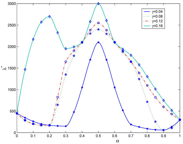
Figure 6. The quantity λ*(α) as a function of the parameter α for several choices of the threshold γ (Criterion 1).
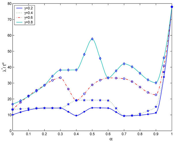
Figure 7. The quantity λ*(α)/tα as a function of the parameter α for several choices of the threshold γ (Criterion 2).
choice as the corresponding choice when we use Criterion 1. However, for example, Figures 6 and 7 show that the choice α = 0.5 defines a highly performing network for both Criteria.
Figure 8 shows the quantities  and
and  as a function of λ for several values of the parameter α, that is for α = 0, 0.3, 0.5, 0.7, 0.9, 1. We note that the quantity
  is approximately constant up to a given value of λ and that after that value of λ starts to increase (see Figure 8). The results shown in Figure 8 suggests that the networks with α ∈ (0.3, 0.7) are the best performing ones between those studied when we use the quantities NL and tM to judge the traffic quality. In fact in Figure 8 we can see that for λ ∈ [100, 1100] when α = 0.3, 0.5, 0.7 the values taken by the quantities
  and
and  are smaller than the corresponding values of the same quantities when we have α = 0, 0.9, 1.
Let us study some analogies between the network congestion phenomenon considered here and the phase transition phenomenon studied in statistical mechanics using the random variable , that is the number of

Figure 8. The quantities  and
and  as a function of λ for several choices of α.
packets that are travelling on the network minus λtα. Note that the expected value of  is
is . We perform the statistical analysis of
 , that is we approximate the probability density function of
  with the empirical distribution of the simulated data as a function of the parameters α and λ in order to establish the existence of a sizable probability of having a large congestion and we compare the results obtained in this way with those obtained using the Criteria introduced above to study criticality.
For several choices of the parameters α and λ we perform a number of simulations sufficient to obtain an empirical approximation of the probability density function of . When α = 0, Figures 9 and 10 show the empirical probability density functions obtained, that is they show the relative frequencies of
  obtained in the simulations for a fixed value of the mean load λ, that is for λ = 30, 300, 3000 and 6000.
Let  be a lower and an upper bound respectively for the critical value λ* of the parameter λ. When α = 0 a sign of congestion appears when the (empirical) probability density function of
  changes its form from being a unimodal function independent of time peaked around zero (for λ ≤
 , see Figure 9) to being a bi-modal function that translates to the right when time goes on (for λ ≥
 , see Figure 10 where the probability density functions obtained for t = T are shown). Looking at Figures 9 and 10, we can see that
  should have a value smaller than λ = 3000 and greater than λ = 300 (it seems reasonable to be conservative and choose
  = 300) and that
  should have a value greater or equal than 3000 and smaller or equal than 6000 (it seems reasonable to be conservative and choose
  = 3000). In fact, Figure 10 shows that when λ ≥ 3000 the empirical probability density function of
  is not peaked in zero (i.e. the number
  is substantially greater than the value λtα which is the approximate value of
  in the free flow state in stationary conditions). We can conclude that the phase transition from the free flow regime to the congested regime takes place for a value of λ belonging to the interval [
 ]. Indeed, more refined numerical simulations have shown that the interval [
 ] can be reduced to the interval: [500, 600]. Note that this is in substantial agreement with the critical value of λ for the network Inet 3037 determined using Criterion 1 (see Figure 6).
Figure 11 shows the empirical probability density function of  for α = 0.5 when λ = 300 (Figure 11(a)) and λ = 3000 (Figure 11(b)). Let us compare Figure 9(b), 11(a) (i.e. λ = 300) and Figure 10(a), 11(b) (i.e. λ = 3000). Note that when α = 0.5 (i.e. Figures 11(a) and (b)) the empirical probability density function of
  is peaked in zero and the frequency corresponding to the window containing zero is approximately 70% (λ = 300) or 60% (λ = 3000) and that when α = 0 (see Figure 9(b)) the empirical probability density function of
  is peaked in zero and that the frequency corresponding to the window containing zero is approximately 35% (λ = 300), moreover when α = 0 and λ = 3000, the probability density function of
  is not peaked in zero (see Figure 10 (a)). This fact suggests that the α = 0-network starts changing regime earlier than the α = 0.5-network, that is we should expect that the α = 0-network reaches the congested regime for a smaller value of the load parameter λ than the α = 0.5-network. This is confirmed by the analysis done using Criterion 1
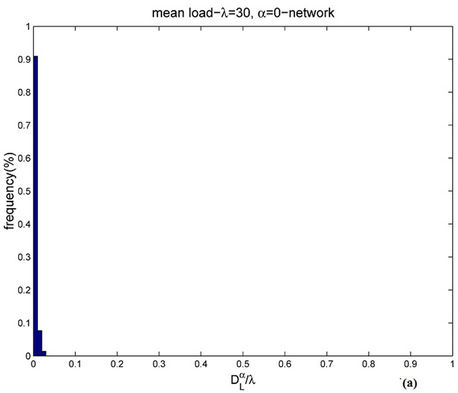

Figure 9. Frequency distribution of  when α = 0 and λ = 30 (a) or λ = 300 (b).
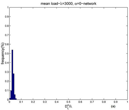

Figure 10. Frequency distribution of  when when α = 0 and λ = 3000 (a) or λ = 6000 (b).
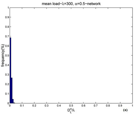
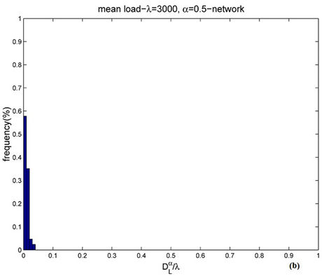
Figure 11. Frequency distribution of  when α = 0.5 and λ = 300 (a) or λ = 3000 (b).
and 2 (see Figures 6 and 7). Let us study the congestion phenomenon from a different point of view. Let us consider the function , λ > 0. From the behaviour of
 , λ > 0, shown in Figure 8 it is reasonable to assume that zα(λ) as a function of λ behaves as follows:
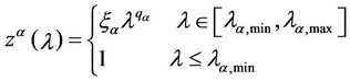 , (12)
where ξα is a positive constant depending on the network topology, qα is a negative exponent, λα,min, λα,max are, respectively, a lower and an upper bound defining an interval where the transition from the free flow to the congested regime takes place. This transition from the free flow to the congested regime can be assimilated to the phase transition phenomenon studied in statistical mechanics. Equation (12) is motivated by the fact that when the network has not reached the congested regime  is approximately equal to tα and the probability density function of
  is peaked in zero. On the contrary when the network has reached the congested regime we have that
  increases with λ and that the probability density function of
  is not peaked in zero. Note that when λ is greater than λ* (remember that λ* < λα,max) the network does not have a stationary regime (in time) anymore and the quantities
  and
and  are not defined, in fact they diverge with time. That is in this last case the quantities
 ,
,  shown in the figures are those observed at time T, the time where the numerical simulation ends.
We choose λα,max = 3000 and we calibrate the parameters qα, ξα, λα,min appearing in formula (12) from the simulation data relative to the function zα(λ) using a least squares procedure. Let us denote with  the relative mean square error at the solution of the least squares procedure. Figures 12(a), (b), (c), (d) show the error
  as a function of λα,min when α = 0, α = 0.5, α = 0.7 and α = 1 respectively. Note that all the functions
  (λα,min), λα,min > 0, shown in Figure 12 have a local minimizer except the one shown in Figure 12(d) that is relative to the α = 1-network. Remind that the α = 1-network corresponds to the modified rectangular lattice. The existence of a local minimizer indicates the transition from the free flow regime to the congested regime. In fact, when λ is sufficiently large the function
  decreases monotonically and behaves like
  so that increasing λα,min we can improve the matching of the simulated data with the curve given in (12). Let [λα,min, λα,max] be the interval where the function zα(λ), as a function of λ behaves as a negative power. For α = 0, α = 0.1·i, i = 2, 3, ∙∙∙, 7, α = 0.9, we can observe that the transition from a free flow regime to a congested regime (according with Criterion 2) is located in the interval [
 , λα,max] when we choose
  to be the first local minimizer of
  (see Figure 12). Table 3 shows the parameters obtained using the calibration procedure described above and choosing λα,min=
 . We improve the choice of λα,min, λα,max made previously to obtain an interval of criticality [
 ] smaller than the interval [λα,min, λα,max]. A possible choice of the interval [
 ] is
] is  and
and , where
  is the largest value of λ such that we have
 , α = 0, α = 0.1·i, i = 2, 3, ∙∙∙, 7, α = 0.9.
Finally Figure 12(d) shows that when α = 1 the phase transition does not occur for the values of λ considered in the simulations. In fact, in the modified rectangular lattice network (i.e. α = 1), the congestion phenomenon takes place for greater values of λ than those considered in the numerical simulation presented here. That is the modified rectangular lattice has a free flow region greater than that of the remaining networks considered. This desirable property is obtained at the price of a delivery time in the free flow regime approximately seven times greater than the delivery time of the other networks considered. Note that Figure 8 shows that the delivery time of the modified rectangular lattice network is constant in the interval of λ considered and is bigger than the biggest delivery time of the remaining α-networks.
Table 3 shows that the exponent qα obtained from the least squares procedure takes substantially three different values: qα ≈ −0.5333 for α = 0, qα ≈ −0.6 for α = 0.2, 0.3, 0.4 and qα ≈ −0.64 for α = 0.5, 0.6, 0.7, 0.9. These numerical findings and Table 4 suggest that the exponent qα depends from the maximum value of the weighted betweenness centrality,  , with respect to the node index v. It will be interesting to investigate more deeply the existence and eventually the meaning of this relation. We do not pursue this investigation in this paper.
Our analysis shows that when the load λ increases the traffic flow on the network first tries to continue to deliver all the packets increasing the delivery time of each packet and then starts to leave some packets undelivered. In fact Figure 8 shows that even when the increment of the mean travel time , α ∈ [0, 1) is relevant (see, for example, the interval λ ∈ [150, 300]) the corresponding value of
 , α ∈ [0, 1) is approximately zero. That is, for α ∈ [0, 1) the α-network starts to undeliver packets only when the mean travel time is becoming at least twice the (approximate) delivery time tα of the free flow regime. The behaviour of the modified rectangular lattice (α = 1) is different from the behaviour of the remaining networks. This is probably due to the fact that when we go from α ∈ [0, 1) to α = 1 the rich club vanishes. As a consequence for α = 1 the delivery time remains substantially unchanged even for large values of λ, but there is a significative quantity of undelivered packets. In fact, when α ∈ [0, 1), due to the choice of the routing strategy, the majority of
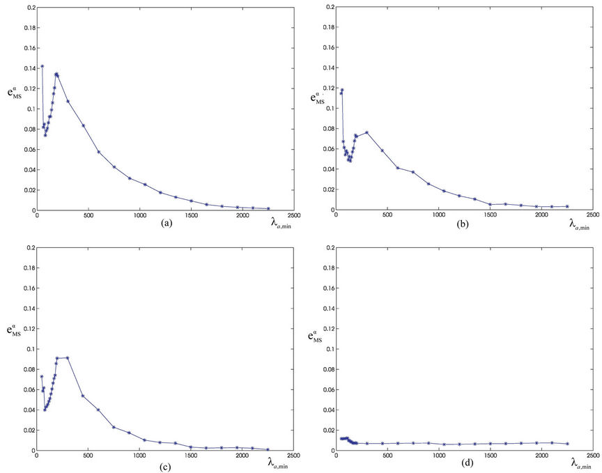
Figure 12. Relative least square error as a function of λα,min when α = 0 (a), α = 0.5 (b), α = 0.7 (c) and α = 1 (d).
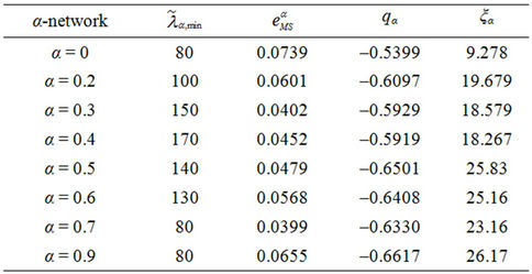
Table 3. Parameter calibration.
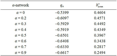
Table 4. Relation between the exponent qα and the maximum weighted betweenness centrality  as a function of the node index v.
the packets go to their destination passing through the rich club. This is due to the high weighted betweenness centrality and to the high degree of the nodes of the rich club. When a group of packets go through nodes whose incoming branches have capacities insufficient to deliver them the delivery time increases due to the time spent by the packets waiting in the nodes queues. That is for α ∈ [0, 1) only when the rich club becomes congested the packets start to be undelivered and the delivery time increases substantially (see Figure 8 α = 0, α = 0.9). When α = 1, that is in the modified rectangular lattice, the rich club does not exist anymore and the capacities of all the branches are equal. So that for λ sufficiently large in the modified rectangular lattice in every node there is a small congestion that produces a few undelivered packets and the number of these undelivered packets grows slowly. Table 5 proposes an analogy between the phase transition phenomenon in statistical mechanics and the congestion phenomenon studied here. This analogy summarizes some of the facts explained in this section. More general results about network analysis based on the analogies between network behaviour and statistical mechanics can be found in [16,17].
We conclude this Section noting that Figures 6, 7, 8
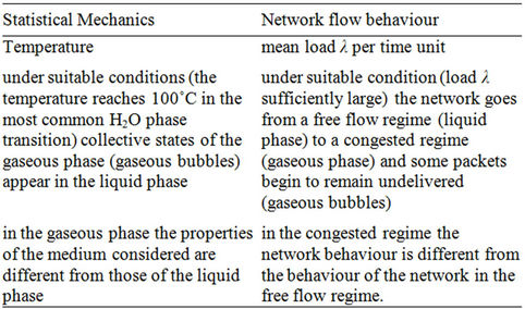
Table 5. Analogies between the phase transition phenomenon in statistical mechanics and the network traffic congestion phenomenon.
and Table 3 show that the curves  as a function of λ for α ∈ (0.3, 0.7) are the smallest ones between those considered and that this is also true for the expected value of
 , that is for
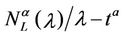 . From these facts we can say that the choice of the parameter α in the interval (0.3, 0.7) defines a set of networks that is an interesting compromise between Inet 3037 (α = 0) and the modified rectangular lattice network (α = 1).
4. The Traffic Congestion Phenomenon in the Heterogeneous Traffic Case
Let us study the congestion phenomenon in the heterogenous traffic case. As already mentioned in the Introduction we study on the networks considered previously the traffic of three different kinds of data packets. We consider three different traffic situations assigning different values to the constants βj, j = 1, 2, 3, that defines the mean load βiλ of the packets of kind i, i = 1, 2, 3. That is we consider the following cases:
Case (a): β1 = β2 = β3 = 1/3. This is a balanced load situation and generates a load per unit time having in average the same number of packets for the three kinds of packets;
Case (b): β1 = 5/7, β2 = 1/7, β3 = 1/7. This is an unbalanced load situation and generates a load per unit time having in average a large number of packets with highest priority (kind i = 1), the remaining two kinds of packets have in average a smaller number of packets and in particular since β2 = β3 they have the same number of packets;
Case (c): β1 = 1/6, β2 = 2/6, β3 = 3/6. This is the most common load situation, that is the situation where the number of packets per unit time with the highest priority (kind i = 1) is (in average) smaller than the number of packets per unit time of intermediate priority (kind i = 2) and this last number is (in average) smaller than the number of packets per unit time with lowest priority (kind i = 3).
The simulation procedure in the heterogeneous traffic case is similar to the simulation procedure in the homogeneous traffic case described in Section 3 except for Step 4, packet generation, and Step 6, queue management, that must be adapted to the new situation.
The simulation procedure in the heterogeneous traffic case can be summarized in the following steps:
1) the same as Step 1 of the analogous procedure of Section 3;
2) the same as Step 2 of the analogous procedure of Section 3;
3) the same as Step 3 of the analogous procedure of Section 3;
4) packets generation: given βj ≥ 0, j = 1, 2, 3, such that
 in each time unit of the simulation the number of kind i packets generated is sampled from a Poisson random variable with parameter βiλ, i = 1, 2, 3, where λ is a positive parameter. The values of λ considered in the simulations are 201 values equispaced in the interval [2, 3600], that is we choose λ = λk = 2 + (3600−2)k/200, k = 0, 1, ∙∙∙, 200. To each packet generated is assigned a couple of nodes. This couple of nodes is sampled from a random variable uniformly distributed on the set of the couples (s, d) such that s ≠ d, s, d = 1, 2, ∙∙∙, 3037. The packet associated to a couple of nodes originates in the first element of the couple and has destination in the the second element of the couple. The packets of kind i have priority pi, i = 1, 2, 3. In the numerical simulations we choose: p1 = 3, p2 = 2, p3 = 1;
5) routing strategy: the same as in Step 5 of the analogous procedure of Section 3;
6) queue management: every node has a queue for each branch (of positive capacity) leaving the node that we assume potentially unbounded. When a packet arrives or is generated at a node, it is placed in the appropriate queue of the node to be delivered toward its destination along its route. The queue management rule consists in the choice of moving first the packet having the largest product waiting time at the node times priority factor. When two or more packets have the largest product waiting time at the node times priority factor we deliver first the packet that has been generated earlier. If at a node two or more packets having the largest waiting time times priority factor have been generated at the same time we choose randomly between them the packet to move first. When two or more packets present at a node must continue their route along the same branch and there is sufficient capacity available on the branch the packets go in the same time unit through the branch;
7) packets movement: the same as in Step 7 of the analogous procedure of Section 3.
Let ,
, , λ > 0, α ∈ [0, 1], i = 1, 2, 3, be the functions defined in the Introduction. To study the congestion phenomenon in the heterogeneous traffic case we must generalize Criterion 1 and 2 used in Section 3 in the homogeneous traffic case to study criticality. This is done as follows:
Criterion 3: Given an α-network and the constants βj ≥ 0, j = 1, 2, 3, such that , for i = 1, 2, 3, we say that
  is the critical value of the load parameter λ for the α-network and the kind i data packets when
  is the smallest value of λ such that the derivative with respect to λ of
  measured using λ as unit, that is the quantity
 , is greater than a given positive constant γ.
Criterion 4: Given an α-network and the constants βj ≥ 0, j = 1, 2, 3, such that , for i = 1, 2, 3, we say that
  is the critical value of the load parameter λ for the α-network and the kind i data packets when
  is the smallest value of λ such that the derivative with respect to λ of the mean travel time measured using tα as unit, that is the quantity
 , is greater than a given positive constant γ.
The value assigned to the constant γ in the numerical simulations will be specified later.
The numerical simulation shows that in Case (a) and Case (c) the curves that represent the quantities  and
and  as a function λ, i = 1, 2, 3 do not intersect. In fact we have:

 (13)
(13)
That is, in Case (a) and Case (c), by virtue of (13) we have . However in Case (b) the behaviour of the quantities
  as a function of λ, i = 1, 2, 3, is not that simple and depends on the network considered, that is it depends on α, α ∈ [0, 1]. Let us be more specific.
Figures 13, 16, 19 show the quantities , i = 1, 2, 3, as a function of the parameter λ when the network studied is Inet 3037 (α = 0) in the load situation described by Case (a), Case (b) and Case (c) respectively.
Figures 14, 17, 20 show the quantities ,
,  , i = 1, 2, 3, as a function of the parameter λ when the network studied is the α = 0.5-network in the load situation described by Case (a), Case (b) and Case (c) respectively.
Figures 15, 18, 21 show the quantities ,
,  , i = 1, 2, 3, as a function of the parameter λ when the network studied is the α = 0.9999-network in the load situation described by Case (a), Case (b) and Case (c) respectively.
Looking at Figures 13-21 we can see that, in Case (a) and Case (c), the kind 1 packets behave approximately like the other kinds of packets and the inequalities (13) are satisfied. We note that when we consider Inet 3037 (α = 0) and the α = 0.5-network the kind 1 packets reach the

Figure 13. The quantities  and
and  as a function of λ, i = 1, 2, 3, when α = 0 and β1 = β2 = β3 = 1/3.

Figure 14. The quantities  and
and  as a function of λ, i = 1, 2, 3, when α = 0.5 and β1 = β2 = β3 = 1/3.
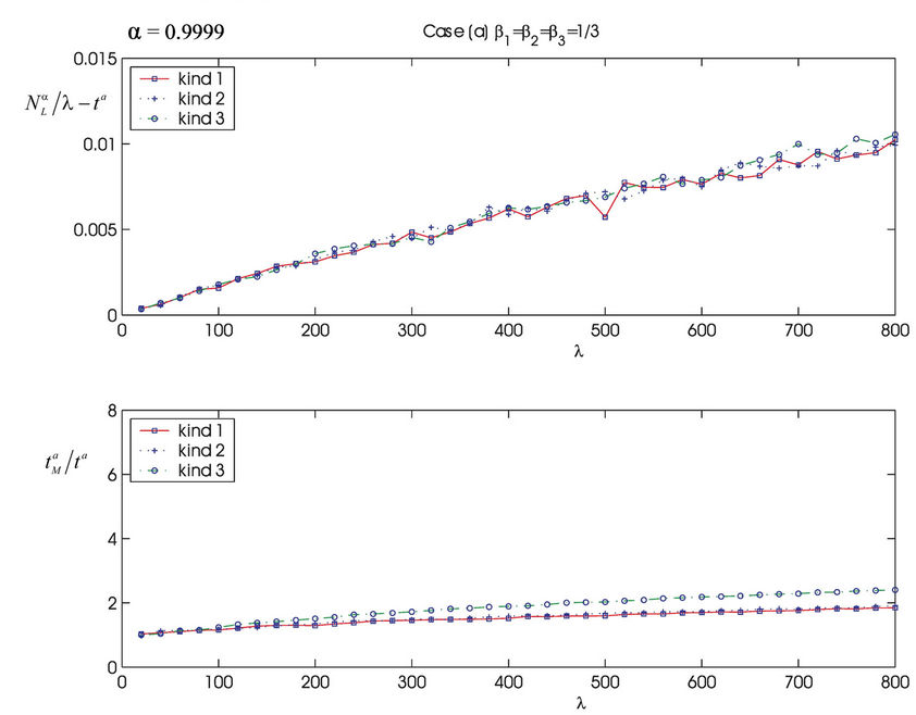
Figure 15. The quantities , and
, and  as a function of λ, i = 1, 2, 3, when α = 0.9999 and β1 = β2 = β3 = 1/3.

Figure 16. The quantities , and
, and  as a function of λ, i = 1, 2, 3, when α = 0 and β1 = 5/7, β2 = β3 = 1/7.

Figure 17. The quantities , and
, and  as a function of λ, i = 1, 2, 3, when α = 0.5 and β1 = 5/7, β2 = β3 = 1/7.

Figure 18. The quantities , and
, and  as a function of λ, i = 1, 2, 3, when α = 0.9999 and β1 = 5/7, β2 = β3 = 1/7.
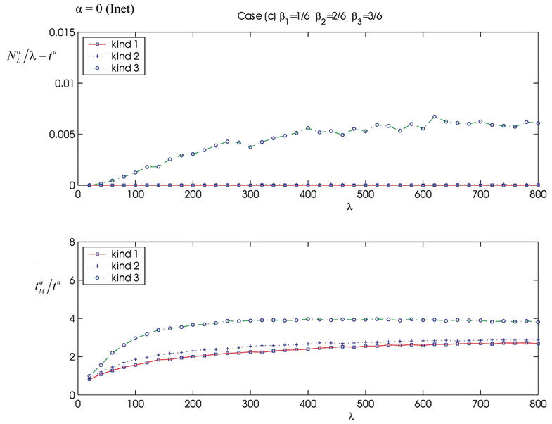
Figure 19. The quantities , and
, and  as a function of λ, i = 1, 2, 3, when α = 0 and β1 = 1/6, β2 = 2/6, β3 = 3/6.

Figure 20. The quantities , and
, and  as a function of λ, i = 1, 2, 3, when α = 0.5 and β1 = 1/6, β2 = 2/6, β3 = 3/6.

Figure 21. The quantities , and
, and  as a function of λ, i = 1, 2, 3, when α = 0.9999 and β1 = 1/6, β2 = 2/6, β3 = 3/6.
criticality after the other kinds of packets in all Cases (a), (b), (c) when we apply Criterion 4. However when we use Criterion 3 and we consider Case (b) the kind 1 packets reach criticality before the remaining kinds of packets.
The traffic on the α = 0.9999-network is substantially different. In particular it seems that, in the balanced load condition (Case (a)) and in the usual load condition (Case (c)) the kind 1 packets behave as the remaining kinds of packets. That is, in the α = 0.9999-network the priorities assigned to the different kinds of packets seem to have a small effect. In fact when α = 0.9999 if we compare the values assumed by  in the homogenous traffic case to the values assumed by
  in the heterogeneous traffic case for kind i packets, i = 1, 2, 3, we can see that they are approximately the same (see Figures 15, 18 and 21). Moreover, in the unbalanced load condition described by Case (b) we observe that the number of undelivered kind 1 packets is greater than the number of undelivered packets of kind 1 and 2. The fact that the effect of the priorities on the traffic of the α = 0.9999-network in term of the delivery of the packets is almost negligible can be attributed to the following facts: the absence of a rich club and the fact that the capacities of all the branches are equal. Note that these two facts are true only for the α = 1-network (modified rectangular lattice) and that they are only approximately true for the α = 0.9999-network. In fact, on the α = 0.9999-network most of the shortest weighted paths do not go through the rich club, that is the packets move between nodes following their routes and they are not attracted by the nodes of the rich club where the priority plays a fundamental role in the queue management. The effect of the priorities in a lattice-like network (α = 0.9999, α = 1) is significant only for larger values of the parameter λ (see Table 7). In the free flow regime the traffic behavior on the α = 0.9999-network is very similar for the three different kinds of packets and the travel times of the three kinds of packets remain substantially the same as the travel time observed in the free flow regime for the homogeneous traffic case.
Let us consider the traffic behaviour on Inet 3037 and on the α = 0.5-network. We can see that, in the Case (a) load situation it is difficult to establish which one of the networks has the best performance. In fact both Inet 3037 and the α = 0.5-network in the region of λ explored are well performing networks for packets of kind 1 and 2 while they penalize the packets of kind 3.
Moreover, looking at Inet 3037, the packets of kind 1 and 2 have mean travel times that are at most 3 times the mean travel time of the free flow regime, while the mean travel time of the kind 3 packets is up to six times the mean travel time of the free flow regime.
Figures 13-21 show that going from the α = 0 to the α = 0.9999-network the role played by the priorities decreases. In fact in all the situations considered when α = 0 the curves corresponding to the three kinds of packets are well separated (i.e. the priorities are working), when α = 0.5 only the curve of the kind 3 packets is well separated from the remaining ones (i.e. the priorities of the first two kinds of packets reduce their role) and when α = 0.9999, as already mentioned, there is no substantial difference in the three curves except for the Case (b) load situation.
Let us look more closely to the Case (b) load situation and let us try to establish an analogy between the traffic associated to Case (b) and the so called thermodynamical triple point.
In thermodynamics, the triple point of a substance is the temperature and the pressure such that three phases (for example, gaseous, liquid, and solid phase) of the substance coexist in thermodynamic equilibrium. For example let us consider H2O (see [18]) as the substance, the combination of pressure and temperature such that water, ice, and water vapor can coexist in a stable equilibrium occurs at a temperature of 273.16 K and a vapor pressure of 611.73 Pascals. In that circumstance, it is possible to change all the water present in the experiment in one of the three phases ice, water, and water vapor by making arbitrarily small changes in pressure and temperature.
In our context the three kinds of packets play the role of the three phases. For example, we can image the kind 1 packets as the gaseous phase due to their greater possibility of moving in the network because of their highest priority, the kind 2 packets as the liquid phase due to their intermediate possibility of moving in the network and, finally, the kind 3 packets as the solid phase since these packets are those whose movement in the network is less easy. The role of the temperature is played by the parameter λ and the role of the pressure is played by the parameter α. Given the choice of the parameters βj, j = 1, 2, 3, the curves , α ∈ [0, 1], i = 1, 2, 3, determine the critical temperatures that separate the phases one from the others as a function of the pressure (i.e. the value of α). In practice for each kind of packets the curve
 , α ∈ [0, 1] represents the curve such that below it we have the free regime and above it we have the congested regime, i = 1, 2, 3.
However under suitable “pressure and temperature conditions” (i.e. a suitable choice of  and
and ) we can observe that all the phases coexist, i.e. we have:
 .
.
Given the load condition (that is given βi, i = 1, 2, 3) the knowledge of the “triple point temperature and pressure” ,
,  is interesting, in fact the knowledge of this “triple point temperature and pressure” makes possible to design slightly modified networks that at that “temperature” operate with the three kinds of packets at the same time in a traffic condition in the free flow regime just below the transition to a congested regime. In this condition the
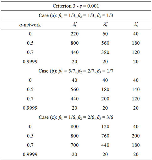
Table 6. Critical value of λ obtained applying Criterion 3 with γ = 0.001 for several values of parameter α ∈ [0, 1] and for each data packet kind ( kind 1,
  kind 2,
  kind 3).
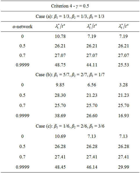
Table 7. Critical value of λ/ obtained applying Criterion 4 with γ = 0.5 for several values of parameter α ∈ [0, 1] and for each data packet kind (
 kind 1,
  kind 2,
  kind 3).
network is fully exploited.
Table 6 shows the critical values  of λ, i = 1, 2, 3, as a function of the parameter α when we use Criterion 3 with γ = 0.001 for the three choices of the parameters βi, i = 1, 2, 3, considered (Case (a), (b), (c)). Table 7 shows the critical values
  of λ, i = 1, 2, 3, divided by the mean travel time as a function of the parameter α when we use Criterion 4 with γ = 0.5 for the three choices of the parameters βi, i = 1, 2, 3, considered (Case (a), (b), (c)). The behaviour of the critical values
 , α ∈ [0, 1], i = 1, 2, 3, shown in Tables 6 and 7 confirms the conclusions reached discussing Figures 13-21.
Figure 22 shows the critical values  of λ, i = 1, 2, 3, divided by the mean travel time as a function of the parameter α when we use Criterion 4 with the threshold γ equal to 0.4. We note that the three curves
 , α ∈ [0, 1], i = 1, 2, 3, shown in Figure 22 delimit a bounded polygonal region. This situation is somehow similar to the thermodynamical triple point phenomenon. Note that in the thermodynamical triple point phenomenon the polygonal region delimited reduces to a point.
We conclude this section with a numerical experiment analogous to an experiment proposed in Section 3. Let us consider the function , λ > 0, i = 1, 2, 3. Let us assume that
 , i = 1, 2, 3, as a function of λ behaves as follows:
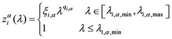 , i = 1, 2, 3, (14)
where ξi,α is a positive constant, qi,α is a negative exponent, λi,α,min, λi,α,max are, respectively, the lower and upper bounds of the interval where for the kind i packets the transition from a free flow regime to a congested regime takes place, i = 1, 2, 3.
Equation (14) can be justified reasoning as done in Section 3 to justify equation (12). For i = 1, 2, 3 we choose λi,α,max = 800 and we calibrate the parameters qi,α, ξi,α, λi,α,min appearing in formula (14) starting from the simulation data relative to the function  using a least squares procedure.
Tables 8 and 9 show some of the results obtained. In particular Table 9 shows that the exponents qi,α, i = 1, 2, 3, seem to be independent of the data packet kind and, depend substantially only on the network topology. On the contrary the values of the parameters λi,α,min, i = 1, 2, 3, in Table 8 seems to be dependent on the data packet kind and on the choice of the values of the constants βj, j = 1, 2, 3. We can conclude that the network topology and the load condition (given by the choice of the values of the quantities βj, j = 1, 2, 3) play an important role in the traffic congestion phenomenon in the heterogeneous traffic case.
5. Conclusions
In this paper a study of the congestion phenomenon for

Table 8. Calibration of the parameters λi,α,min, i = 1, 2, 3.
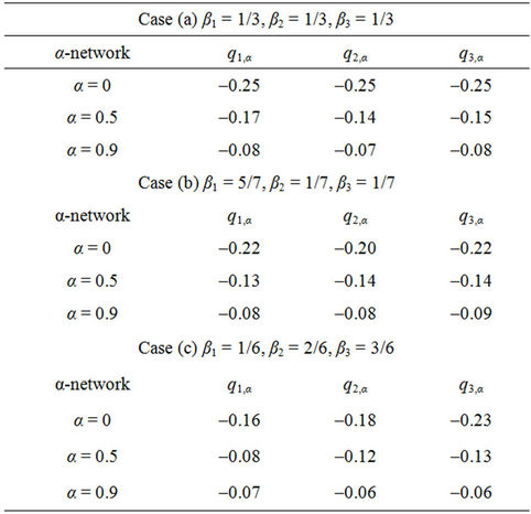
Table 9. Calibration of the parameters qi,α, i = 1, 2, 3.
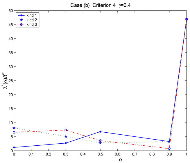
Figure 22. The quantities λi*(α)/tα as a function of the parameter α, i = 1, 2, 3, according to Criterion 4 (Case (b): β1 = 5/7, β2 = 1/7, β3 = 1/7).
homogeneous and heterogeneous traffic of data packets in complex transmission networks is presented. We consider a class of complex networks that we call α-networks, that consists of networks whose topology is obtained by an “interpolation” between the topology of a network having the small world property (i.e.: α = 0) and the topology of a (modified) lattice network (i.e.: α = 1) changing the capacities of the branches. We assume that there are three kind of packets flowing on the α-networks and for i = 1, 2, 3 we find a load critical value  corresponding to packets of kind i. The study of the load critical value
 , α ∈ [0, 1], shows that there exist intermediate network topologies corresponding to suitable choice of the parameters
 , 0 <
, 0 <  < 1, i = 1, 2, 3, that are reasonable compromises from the data packets traffic properties point of view between the network having the small world property (i.e. Inet 3037 in our study) and the modified lattice network (i.e. the modified rectangular lattice in our study). In particular for i = 1, 2, 3 the topology corresponding to
  can be characterized as the topology with the greatest mean load critical value for packets of kind i when we require the mean travel time of the packets of kind i to be smaller than a given quantity. In fact, a well behaved network should guarantee a traffic flow characterized by a reasonably small mean travel time and by a region of free traffic flow as big as possible. Hence for i = 1, 2, 3 the network corresponding to the choice
 , for the kind i packets, absorbs a traffic load greater than the traffic load absorbed by a network having the small world property (i.e.: α = 0) before becoming congested and delivers the packets travelling on the network to their destination in a mean travel time smaller than the mean travel time observed on the corresponding lattice network (i.e.: α = 1) that handles the same load (see Figures 6-8 and Figures 13-21 where we consider α = 0, 0.5, 0.9999). We call these networks
  -networks, i = 1, 2, 3.
Moreover the analysis presented in this paper shows, in the heterogeneous traffic case, an interesting relation between the balance of the load between the different kinds of packets and the critical load values. When the quantities βj, j = 1, 2, 3, are such that β1 < β2 < β3 we have , α ∈ [0, 1], that is the critical values
  as a function of α ∈ [0, 1], i = 1, 2, 3, are three curves that do not intersect each other in the (α, λ) plane. These inequalities between critical values correspond to the fact that when the load increases, that is when λ increases, for α ∈ [0, 1] the traffic with lowest priority gets congested first, followed by the traffic of intermediate priority and finally by the traffic of highest priority. This is the most usual traffic condition on real networks. However when the choice of the quantities βj, j = 1, 2, 3, does not satisfy the inequalities β1 < β2 < β3, and in particular when we have β2 ≤ β3 < β1 the three curves that represent the critical values
 , α ∈ [0, 1], i = 1, 2, 3, in the (α, λ) plane may have intersections in fact the inequalities
  may not hold everywhere for α ∈ [0, 1]. This is an anomalous traffic condition for the network. Some analogies inspired by this last fact between the congestion phenomenon of data packet traffic on networks and the phase transition phenomenon studied in statistical mechanics have been discussed.
REFERENCES
- A. Farina, A. Graziano, F. Mariani and F. Zirilli, “Probabilistic Analysis of Failures in Power Transmission Networks and Phase Transitions: a Study Case of a High Voltage Power Transmission Network,” Journal of Optimization Theory and Applications, Vol. 139, No. 1, 2008, pp. 171-199. doi:10.1007/s10957-008-9435-x
- L. Kocarev and G. Vattay, “Complex Dynamics in Communication Networks,” Springer Verlag, Berlin, 2005. doi:10.1007/b94627
- W. Aiello, F. Chung and L. Lu, “Random Evolution in Massive Graphs,” In: J. Abello, P. M. Pardalos and M. G. C. Resende, Eds., Handbook of Massive Data Sets, Kluwer Academic Publisher, Norwell, 2002, pp. 97-122.
- A. L. Fabrikant, E. Koutsoupias and C. Papadimitriou, “Heuristically Optimized Trade-offs: A New Paradigm for Power Law in the Internet,” In: P. Widmayer, F. Triquero, R. Morales, M. Hennessy, S. Eidenbenz and R. Conejo, Eds., Lectures Notes in Computer Science, Springer Verlag, Berlin, 2002, pp. 110-122.
- A. L. Barabasi and R. Albert, “Emergence of Scaling in Random Network,” Science, Vol. 286, No. 5439, 1999, pp. 509-512. doi:10.1126/science.286.5439.509
- S. Jamin and J. Winick, “Inet-3.0: Internet Topology Generator,” University of Michigan, Ann Arbor, 2002.
- A. Medina, A. Lakhina, I. Matta and J. Byers, “BRITE: an Approach to Universal Topology Generation,” 2001. http://www.cs.bu.edu/brite/publications/BriteMascots.pdf
- Y. Aumann and Y. Rabani, “An O(log k) Approximate Min-Cut Max-Flow Theorem and Approximation Algorithm,” SIAM Journal on Computing, Vol. 27, No. 1, 1998, pp. 291-301. doi:10.1137/S0097539794285983
- H. Okamura and P. Seymour, “Multicommodity Flows in Planar Graphs,” Journal of Combinatorial Theory B, Vol. 31, No. 1, 1981, pp. 75-81. doi:10.1016/S0095-8956(81)80012-3
- F. T. Leighton, “Introduction to Parallel Algorithms and Architectures: Arrays, Trees, Hypercubes,” Morgan Kaufmann Publishers, San Francisco, 1992.
- S. Leonardi, “On-line Network Routing,” In: A. Fiat and G. Woeginger, Eds., Online Algorithms—The State of the Art, Springer Verlag, Berlin, 1998, pp. 242-267.
- M. Faloutsos, P. Faloutsos and C. Faloutsos, “On Powerlaw Relationships of the Internet Topology,” ACM/ SIGCOMM Computer Communication Review, Vol. 29, No. 4, 1999, pp. 251-262. doi:10.1145/316194.316229
- L. Subramanian, S. Agarwal, J. Rexford and R. H. Katz, “Characterizing the Internet Hierarchy from Multiple Vantage Points,” 2002. http://research.microsoft.com/en-us/people/sagarwal/infocom02.pdf
- E. W. Dijkstra, “A Note on Two Problems in Connection with Graphs,” Numerische Mathematik, Vol. 1, No. 1, 1959, pp. 269-271. doi:10.1007/BF01386390
- O. Allen, “Probability, Statistics and Queueing Theory with Computer Science Application,” Academic Press, New York, 1990.
- B. Shen and Z. Gao, “Dynamical Properties of Transportation on Complex Networks,” Physica A: Statistical Mechanics and its Applications, Vol. 387, No. 5-6, 2008, pp. 1352-1360. doi:10.1016/j.physa.2007.10.035
- R. D. Smith, “Data Traffic Dynamics and Saturation on a Single Link,” International Journal of Computer and Information Engineering, Vol. 3, No. 1, 2009, pp. 11-16.
- C. J. Adkins, “Equilibrium Thermodynamics,” Cambridge University Press, Cambridge, 1983.
NOTES
*The numerical experience reported in this paper has been obtained using the computing grid of Enea (Roma, Italy). The support and the sponsorship of Enea are gratefully acknowledged.
#The work of this author has been partially supported by SELEX Sistemi Integrati S.p.A. (Roma, Italy) through a research contract granted to CERI-Università di Roma “La Sapienza”.