International Journal of Astronomy and Astrophysics
Vol.3 No.3(2013), Article ID:36514,4 pages DOI:10.4236/ijaa.2013.33032
Study of Duct Characteristics Deduced from Low Latitude Ground Observations of Day-Time Whistler at Jammu
Department of Physics, National Institute of Technology, Srinagar, India
Email: altafnig@rediffmail.com
Copyright © 2013 M. Altaf, M. M. Ahmad. This is an open access article distributed under the Creative Commons Attribution License, which permits unrestricted use, distribution, and reproduction in any medium, provided the original work is properly cited.
Received February 28, 2013; revised March 30, 2013; accepted April 8, 2013
Keywords: Electron Density; Dispersion; Duct Whistlers; Ionosphere
ABSTRACT
Propagation characteristics of low latitude whistler duct characteristics have been investigated based on day-time measurements at Jammu. The morphogical characteristics of low latitude whistlers are discussed and compared with characteristics of middle and high latitude whistlers. The Max. electron density (Nm) at the height of the ionosphere obtained from whistler dispersion comes out to be higher than that of the background which is in accordance with the characteristics of whistler duct. The equivalent width is found to be close to the satellite observations and the characteristics of whistler duct in low latitude ionosphere are similar to those in middle and high latitude ionosphere. The width of ducts estimated from the diffuseness of the whistler track observed during magnetic storm is found to lie in the range of 50 - 200 Km.
1. Introduction
Ground based whistlers are known to generally attribute to propagate trapped in field aligned whistler ducts at high and middle latitudes [1,2] and also lower latitudes [3,4]. Whistlers which are VLF electromagnetic signals, travel through the ionosphere-magnetosphere coupled system along the geomagnetic field lines to the magnetically conjugate points in the opposite hemisphere have become a very important tool for probing the plasma sphere and beyond. During their propagation through the magnetosphere these whistler waves acquire dispersion characteristic typical of the electron density inhomogenieties present along the whistler path. The physical features and propagation characteristics of low latitude whistlers are the important and interesting subjects in the work of atmospheric research [3]. They found that the propagation characteristics are different with latitude at geomagnetic latitudes less than 40˚. By using the ducted whistlers the dynamics and structure of the magnetospheric thermal plasma have been studied. The phenomena of trapping and propagation of whistlers in ducts has been discussed by many authors [5]. It is universally accepted that because of dependence of the plasma refractive index on the electron density together with its fluctuations and inhomogeniety the focusing of the whistler energy is predominantly due to the presence of ducts of enhanced ionization along the geomagnetic field lines. There is ample indirect experimental evidence to explain the existence of ducts [5-9] explain various low latitude observations demons the existence of the field aligned irregularities in the magnetosphete. Due to the increasing importance and versatility of the whistler technique, it has become obvious that improved understanding of some aspects of whistler propagation in necessary at low latitudes. In Sutu and ground based observations have been used to identify individual ducts. Thus Park and Corpenter [10] have studied how the cross-L diffusion of whistler ducts take place during magnetically disturbed periods. According to Smith and Angerami [11] (1967) the whistler recorded by OGO III shows frequency spectra which enable us to identify different ducts and to measure their size and spacing.
Ray tracing and intensity studies by Tanaka and Hayakawa [12] has theoretically proposed that the ducts with a small scale and with a large enhancement factor should exist in high latitude flank of the equatorial anomaly in order to account for the occurrence of daytime whistlers, ducted propagation seems very plausible from the studies of day-time whistlers [13]. It would necessary for one to conform and elaborate this ducted propagation and examine the properties of day-time ducts, which is the essential importance, is the subject of this paper.
The first direct evidence for the existence of whistler ducts comes from in situ observations on board OGOI [14]. The morphology of the ducts and in particular size and relative enhancement of their electron density are not very well known at present [6,15-17] shows that the duct width varies from 40 - 180 Km during storm time and from 15 - 25 Km during quite times. On the basis of the change in diffuseness, however, Tanaka and Hayakawa [18] have found that the most likely cause of diffuseness is due to the difference in travel time of whistler’s propagation along elementary ducts lying on the inner and outer field line through a duct region, thus supporting the fundamental idea of Crouchley and Finn [19]. The width obtained by the previous others gives indications of the total duct width of the region [18]. We therefore, have studied the morphology of whistler ducts of daytime recorded at our low latitude ground station Jammu, in the hope that we might be able to deduced some supporting ideas, for the conclusions arrived by previous workers.
2. Data Selection
The recording of whistlers at our low latitude ground station Jammu was started in the month of December, 1996 on routine basis. At low latitude, the whistler occurrence rate is low and sporadic. But once it occurs, its occurrence rate becomes comparable to that of mid latitudes [20]. Similar behavior has also been observed at our low latitude Indian station Jammu. For the present study we have chosen some whistlers events recorded during day time at our ground station Jammu on February 14, 1998 as a large number of Whistlers were observed on this day. On February 14, 1998 the spurt in activity started around 1230IST (Indian Standard Time) and lasting for about five hours, ending finally at 1730IST. During this period about 100 whistlers were observed. The period of observation was magnetically quiet with total KP index 1 (Kp ~ 1).
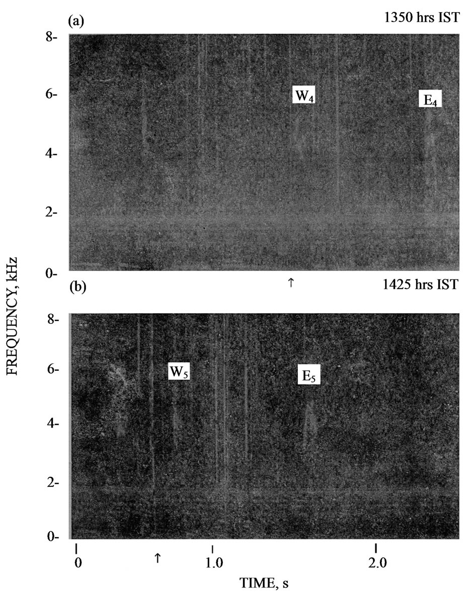
For spectral analysis the normal procedures of analysis by means of sonographic equipment was used. Detailed spectrum analysis has been done for the day time whistlers on February 14, 1998 in order to study the propagation characteristics of these whistlers. From the detailed analysis, it is found that the measured values of recorded whistlers on this day have dispersion of order of 38 sec1/2. The recorded whistlers observed on February 14, 1998 is shown in Figure 1, Figure 2 shows the occurrence histogram of dispersion values for whistler recorded on February 14, 1998 at Jammu.
3. Mathematical Analysis
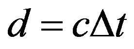
The tweak trace explains the position of whistler source from the observatory is given by the equation.
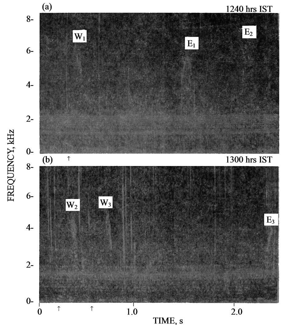
Figure 1. Sonograms as recorded at Jammu on 14 February, 1998 at (a) 1240 hr IST and (b) 1300 hr IST.
 (l)
(l)
where ∆t is the time delay of frequency f = 1.16fc from the front of the tweak here fc = 1.70K Hz is the lower cut-off frequency of the tweak and c is the velocity of light in vacuum. Substituting the values of ∆t in Equation (1) we obtain d = 4650 Km. The distance between the stations and their magnetic conjugate points is about 4745 Km for Jammu. The closeness of the two values of the distance can be taken as an indirect support of the ducted propagation of day-time observed whistlers.
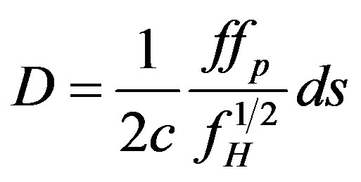
The Max. density of electrons in F-region is calculated from the whistler data and ionospheric sounding. For the quasi longitudinal propagation of VLF electromagnetic waves, the dispersion is related to the parameter of the medium [1].
 (2)
(2)
Here fp fH are the plasma frequency and electron gyro frequency respectively.
We consider that the configuration of the earth’s magnetic field is similar to that of magnetic dip-dipole, for simplicity. Using the equation of magnetic line, we obtain that the Max. height hT of magnetic field line passing through Jammu, is 1158 Km. An ionospheric model with parabolic distribution of electron density is adopted i.e.
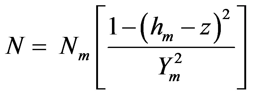 (3)
(3)
where 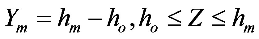
Here hm is the height of Max. electron density of ionosphere, Nm the Max. electron density at hm, Ym, the half thickness of the parabolic ionospheric model and ho the height of the lower boundary of the ionosphere.
From Equations (2) and (3), we obtain
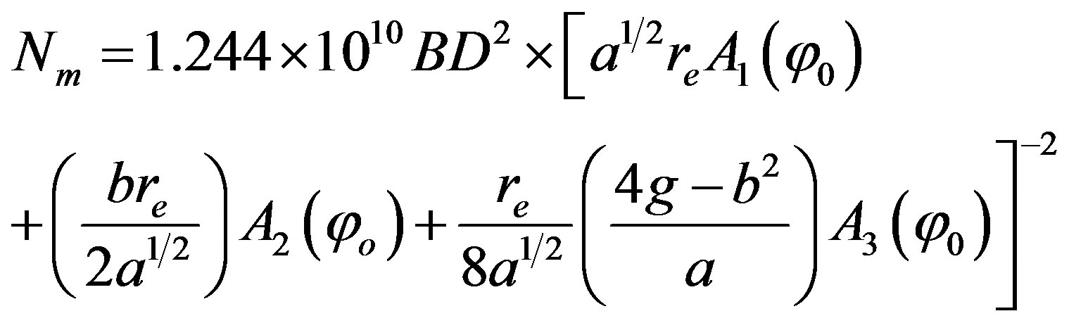 (4)
(4)
where B = geomagnetic induction
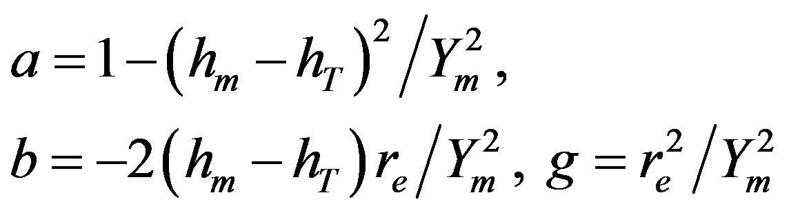
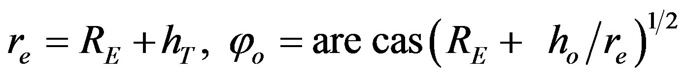
where RE = 6370 Km, the average radius of earth  = 24.33˚N, the magnetic dip latitude of station. By inserting D = 38 secl/2, hm = 283.8 Km, hm = 150 Km, Ym = 133.9 Km and B = 0.38 Guass. We get Nm = 14O × IO5 cm−3 for Jammu. In comparison with Nm = 0.99 × 10 s cm−3 obtained directly from data of ionospheric sounding. The value obtained of Nm from whistler observations to the result is larger by a factor of about one. Thus the electron density along the propagational path of whistler is higher in case of Jammu, which is the characteristic of the whistler duct observed at day-time.
From the width of the trace, the equivalent width of the whistler duct at Max. height of its path can be calculated. By using the definition of dispersion and the Equations (2) and (3) we have
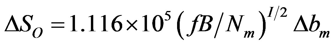 (5)
(5)
where ∆SO is the difference of the equal vent path length and ∆bm is the trace width of the whistler. From the width of the trace at frequency f obtained from the sonograms. ∆SO is calculated, Knowing the latitude of whistler propagation, it is then possible to calculate the effective width of the ducts by using the calculated value of ∆bm from the sonogram. It is found that equal vent width of whistler duct at Max. height of its propagational path is approximately 30 Km estimated from satellite observations (Park, 1980). In some case the width of duct turns out to be approximately 200 Km. This result is in reasonable agreement with that reported by Somayajulu and Tantry (1968) and Okuzawa et al. (1971).
4. Conclusions
The estimation of duct width by using the low latitude whistlers and Satellite observations has been discussed by many workers. In some cases the value is of the order of 80 Km from Satellite observation [21,22]. In some cases its thickness turns out to be approximately 200 Km for stormy days. On quite days the whistler traces are so sharp that the determination of duct width is likely to be in error, because of incoherent limitations in time resolution. Here we have determined the duct width for normal days of day-time duct and it comes out to be 10 - 25 Km which is in good agreement with the results of Somayajulu and Tantry and Okuzawa [6,17].
Hence it has been concluded that the morphological characteristics of low latitude whistlers are same as middle and high latitude whistler. The position of whistler source can be derived from tweak received from Jammu. The Max. electron density of F2-region can be determined from whistler data and ionospheric sounding. The Nm value 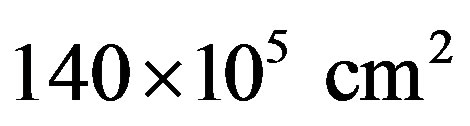 is obtained higher from the whistler dispersion than the background which is the characteristic of the whistler. The equivalent width of whistler duct at the Max. height of its path is found to be very close to the value obtained from satellite observations. It may be shown indirectly that the characteristics of whistler duct in low latitude ionosphere. Duct width estimated from the diffuseness of the whistler traces observed during magnetic storm is found to be in the range of 50 - 200 Km.
5. Acknowledgements
The author is grateful to Director, N I T, Srinagar-190006. Kashmir for his encouragement and keen interest in publishing this research work
REFERENCES
- R. A. Helliwell, “Whistler and Related Ionospheric Phanomena,” Stanfort University Press, Stanfort, 1965.
- R. J. Thomson and R. L. Dowden, “Simultaneous Ground and Satellite Reception of Whistlers I Ducted Whistlers,” Journal of Atmospheric and Solar-Terrestrial Physics, Vol. 39, 1977, pp. 869-877. doi:10.1016/0021-9169(77)90167-2
- M. Hayakawa and Y. Tanaka, “On the Propagation of Low Latitude Whistlers,” Reviews of Geophysics and Space Physics, Vol. 16, 1978, p. Ill.
- M. Hayakawa and K. Ohta, “The Propagation of Low Latitude Whistlers,” Planetary and Space Science, Vol. 40, No. 10, 1992, pp. 1339-1351. doi:10.1016/0032-0633(92)90090-B
- R. I. Smith, “Propagation Characteristic of Whistler Trapped in Field Aligned Column of Enhanced Ionization,” Journal of Geophysical Research, Vol. 66, No. 11, 1961, pp. 3699-3707. doi:10.1029/JZ066i011p03699
- V. V. Somayajulu and B. A. P. Tantry, “Whistlers at Low Latitudes,” J Geomag. Geolect, Vol. 20, 1968, p. 1.
- H. J. Strangeways, “Determination by Ray Tracing of the Region Where Mid Latitude Whistlers Exist from Lower Ionosphere,” Journal of Atmospheric and Solar-Terrestrial Physics, Vol. 43, 1981, pp. 231-238.
- M. Rao and Lalmani, “An Evaluation of Duct Lifetime from Low Latitude Ground Observations of Whistlers,” Planetary and Space Science, Vol. 23, 1975, p. 923.
- J. Lalmani, “Some Aspects of Whistler Duct Lifetimes at Low Latitudes,” Journal of Geophysical Research, Vol. 56, 1984, p. 53.
- S. Wang and Wang, Proceedings of the Conferences on Achievement of the IMS-26-26, June 1984, Graz.
- C. G. Park and D. L. Carpenter, “Whistler Evidence of Large Scale Electron Density Irregularities in the Plasmasphere,” Journal of Geophysical Research, Vol. 75, No. 19, 1970, pp. 3825-3836. doi:10.1029/JA075i019p03825
- R. L. Smith and J. Angrami, “ESSA Conjugate Point Syamposium Institute for Enverimental res. Boulder, Colorade, Vol. 213, 1967.
- Y. Tanaka and M. J. Hayakawa, Journal of Geophysical Research, Vol. 89, p. 755.
- K. Ohta, M. Hayakawa and Y. Tanaka, “Duct Propagation of Daytime Whistlers at Low Latitude as Deduced from Ground Direction Finding,” Journal of Geophysical Research, Vol. 89, 1984, p. 755. doi:10.1029/JA089iA09p07557
- R. I. Smith and J. J. Angerami, “Magnetospheric Properties Deduced from Ogol Observations of Ducted and NonDucted Whistlers,” Journal of Geophysical Research, Vol. 73, 1968, p. 1. doi:10.1029/JA073i001p00001
- J. C. Cerisier, “Ducted and Partly Ducted Propagation of VLF Waves through the Magnetosphere,” Journal of Atmospheric and Solar-Terrestrial Physics, Vol. 36, No. 9, 1974, pp. 1443-1450. doi:10.1016/0021-9169(74)90224-4
- H. J. Strangeways, “Trapping of Whistler Mode Waves in Duct with Tapered Ends,” Journal of Atmospheric and Terrestrial Physics, Vol. 43, No. 10, 1981, pp. 1071-1079. doi:10.1016/0021-9169(81)90022-2
- T. Okuzawa, T. Yoshino and K. Yomanaka, “Characteristics of Low Latitude Whistler Properties Associated with Magnetospheric Storm in March 1970,” Rept.ionosph. Space Rev. Japan, Vol. 25, 1971, p. 17.
- Y. Tanaka and M. Hayakawa, “The Effect of Geomagnetic Disturbances on Duct Propagation of Low Latitude Whistlers,” Journal of Atmospheric and Solar-Terrestrial Physics, Vol. 35, No. 9, 1973, pp. 1699-1703. doi:10.1016/0021-9169(73)90186-4
- J. Crouchley and R. J. Finn, “A Study of Whistling Atmospheric II Diffuseness,” Australian Journal of Physics, Vol. 14, No. 1, 1961, pp. 40-56. doi:10.1071/PH610040
- M. Hayakawa, Y. Tanaka, S. S. Sazhin, M. Tixier and T. Okada, “A Proposal of Daytime Multisationed Direction Finding Measurements of Low and Equatorial Latitude Whistlers in China,” Journal of Geophysical Research, Vol. 93, No. A6, 1988, pp. 5685-5700. doi:10.1029/JA093iA06p05685
- C. G. Park, “Handbook of Atmospherics,” CRC Press, Baca Raton, 1980.