Journal of Minerals and Materials Characterization and Engineering
Vol.1 No.4(2013), Article ID:35103,8 pages DOI:10.4236/jmmce.2013.14029
Analytical Solutions and Computer Simulations of the Evolution of Flat Temperature Profiles in Spherical FRRPP Systems
1Department of Chemical Engineering, Michigan Technological University, Houghton, USA
2Najran University, Najran, Saudi Arabia
Email: caneba@mtu.edu, maaalharthi@nu.edu.sa
Copyright © 2013 Gerard T. Caneba, Mathkar A. Alharthi. This is an open access article distributed under the Creative Commons Attribution License, which permits unrestricted use, distribution, and reproduction in any medium, provided the original work is properly cited.
Received April 8, 2013; revised May 27, 2013; accepted June 14, 2013
Keywords: Flat Temperature Profile; FRRPP; Polymerization; Nonisothermal Reaction; Spherical Reactive Domains; Exponential Integral Function
ABSTRACT
The free-radical retrograde-precipitation (FRRPP) process was recently brought into the quantitative areas of work, based on the discovery of possibility of flat temperature profiles in spherical reactive domain systems. With an approximate decoupling analysis of the energy equation from the component-balance equations, these flat temperature profiles were found to be either stable or unstable. Moreover, resulting evolution of the flat profiles has been found to be expressed analytically through the so-called exponential Integral function, which has been shown to be quantitatively inaccurate during the early times of the process. This work tries to resolve this inaccuracy problem, by comparing the exponential integral results with polynomial approximation and numerical results. The result is that for the stable system, the linearized treatment of the evolution of flat temperature profiles is valid at the early 30% - 40% in the temperature axis, while the remainder of the evolution curve is well-represented by the application of the exponential integral function. For the unstable system, the only thing that can be generalized is that both linear and cubic polynomial approximations are reasonably accurate at very small times and temperatures close to initial values.
1. Introduction
A reactive spherical chain-polymerization particulate system with an exothermic heat of reaction is normally expected to exhibit a parabolic temperature profile, as depicted in Figure 1. In these systems, the idea of a flat temperature profile is almost unheard of, and potentially beneficial in terms of operational and product uniformity. Also, the analysis of the model equations can become less complicated for these types of systems, because a field dynamics problem can be reduced to the relative simplicity of a lumped-parameter system.
In recent publications [1,2], it has been conceptually shown that the so-called free-radical retrograde-precipitation polymerization (FRRPP) process can result in flat temperature profiles through a combination of thermodynamic, transport, and reaction-kinetic parameters in the system. This is shown in Figure 2, wherein the profile starts at a uniform Dimensionless T (or θ in Equation (6)) of 1.0. The temperature profile ends at a steady-state value of Dimensionless T = 1.83 [3]. Note that the dimensionless r in the horizontal axis of Figure 2 is the same as h in Equation (7). This means that the reactive fluid will have h ranging from 0 to 1 only. Values of h between 1 and 2 are rescaled so that they correspond to those of the stagnant fluid boundary layer.
The prediction of the possibility of the occurrence of flat temperature profiles from FRRPP systems has been advanced from a pseudo-steady-state analysis of the energy balance of a model spherical reacting system undergoing polymerization-induced phase separation [1]. The dimensionless differential energy balance has been shown as
 (1)
(1)
and the dimensionless energy source term Φ is expressed as
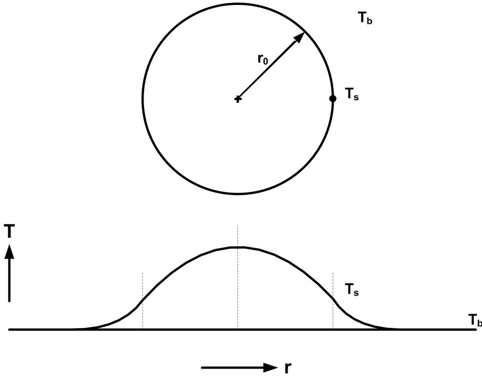
Figure 1. The model used for the analysis of the effect of exotherm when chain polymerization occurs within a spherical particulate system that is immersed in a fluid bath. The uniform fluid bath temperature is Tb and the particulate surface temperature is Ts.
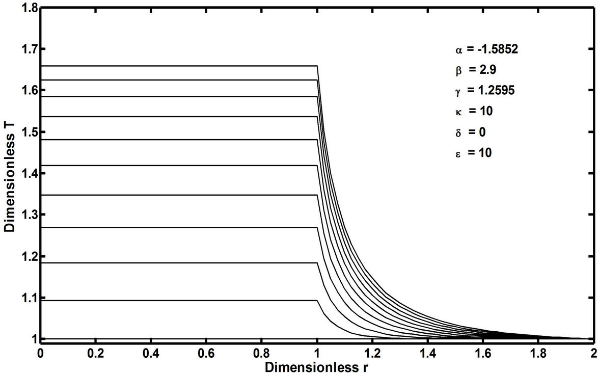
Figure 2. Temperature profile of a chain polymerization FRRPP spherical particulate system along the radial axis, h = r/ro, and with dimensionless time (t in Equation (15)) from 0 to 2.5 stepping up by 0.25. At dimensionless time of 0, the profile starts at a uniform dimensionless T (same as θ in Equation (6)) of 1.0. The temperature profile in the reaction zone (dimensionless r = 0 to 1) ends at a steady state value of dimensionless T = 1.83 [Alharthi, 2010]. For reference, κ is the ratio of the fluid stagnant film thickness to the particulate radius, δ is the thermal conductivity ratio of the fluid to that of the reactive particulate, and ε is the thermal diffusivity ratio of the fluid to that of the reactive particulate.
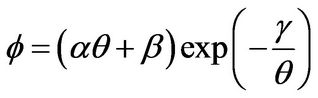 (2)
(2)
The dimensionless parameters are related to the following dimensional quantities in the energy balance and phase equilibria equations:
 (3)
(3)
 (4)
(4)
 (5)
(5)
 (6)
(6)
 (7)
(7)
 (8)
(8)
 (9)
(9)
The phase behavior for the polymer-rich phase was approximated by the linear representation
 (10)
(10)
where XP is the product of the weight fractions of the monomer and polymer (or just the weight fraction of the polymer if the monomer concentration is the same for both polymer-rich and polymer-lean phases at equilibrium, as the case for the PS-S-Ether system [4,5]. Since Equation (10) provides a mesoscopic-macroscopic relationship between the temperature and monomer composition, it allows the decoupling of the mesocopic-macroscopic analysis of the time evolution behavior of the thermal aspect of the system from compositional aspects, until the details of the kinetics of microphase separation behavior is incorporated in the field equations.
In order to quantitatively characterize the relatively lower inefficiency of radical maintenance in free-radical polymerization systems, the expression for XP in Equation (10) can be modified to include a polymer radical efficiency factor fP; thus,
 (11)
(11)
Also, a and b in Equation (10) were proposed to be obtained from experimental data points of phase equilibria experiments. It should be noted that the polymer radical efficiency factor, fP, is related to the initiator efficiency, f, in free-radical polymerizations in a relative sense, i.e., for the same monomer, solvent, their concentrations, and operating temperatures, fP is relatively high when an initiator with a relatively high f is used. The reason is that initiation is the starting point in time when inefficiencies of radical production take place. The survival of propagated radicals will later depend on the effectiveness of the FRRPP radical trapping mechanism, which should result in fP < f. For example, in FRRPP of polystyrene-styrene-ether systems using azobis diisobutylonitrile (AIBN) as initiator, fP was found to be in the order of 0.20 [1,4] even though f was known to be around 0.57 [6].
For the expectation of a flat temperature profile, θ = 1 for η = 0; thus, the dimensionless source term was symbolized as Φo and Equation (2) became
 (12)
(12)
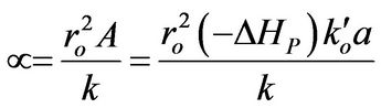
Then, a combined dimensionless quantity was introduced to quantitatively characterize strict FRRPP behavior, wherein the reactive polymer-rich domains attained flat temperature profiles. The dimensionless quantity was symbolized by  (pronounced see-enye), and defined as
 (13)
(13)
Values of  from computational efforts indicated that for the FRRPP process, it should be at least below −1000 for a flat temperature profile [1].
In the unsteady-state analysis of the FRRPP system, the occurrence of the flat temperature profile from FRRPP systems was reinforced, with additional criteria for stability of steady-state behavior [2]. For a stable steady-state system, it was found that the quantity α < 0 even for an insulated reactive domain system. For a > 0, the reactive system was found to be under control with the possibility of a flat temperature profile through relatively ineffective heat removal from the fluid. With more aggressive heat removal from the fluid, the temperature profile in the reactive solid becomes more of a parabolic one.
When the monomer concentration drops to low enough values, the reactive system automatically reverts to a stable one, because the value of α automatically becomes a negative number [1]. This happens either locally (due to relatively fast reaction rate compared to diffusion rate, or polymer domain densification [2]) or in the overall reactive system, due to depletion of monomer molecules.
With assumption of a flat temperature profile, the field energy balance equation was simplified to a mixing-cup ordinary differential equation and later analyzed for its stability characteristics [2]. Results from the field partial differential equation correspond to the reacting sphere with insulated surfaces. An analytical expression for the modified dimensionless temperature (Q) vs dimensionless time (τ) was also obtained for the flat temperature profile reactive spherical domain with insulated boundary surfaces as
 (14)
(14)
in which the dimensionless time was expressed as
 (15)
(15)
and the modified dimensionless temperature (Q), and
and  are obtained as
 (16)
(16)
 (17)
(17)
 (18)
(18)
Note that Tb is the bulk fluid temperature while Ts is the reactive particle surface temperature (Figure 1).
The function, Ei or the Exponential Integral Function [7], is a special transcendental function which has been found to occur in only a few experimental systems; thus,
 (19)
(19)
It can be evaluated through the following infinite series expansion for real positive arguments (x > 0):
 (20)
(20)
The Euler-Mascheroni constant (also called Euler’s constant) has been cited to be equal to 0.5772156649... It should be noted from Equation (20) that the Ei function approaches −∞ at its argument (x) approaching zero from the positive side (0+). This is reflected in inaccuracies in results from direct evaluation Equation (14) at τ → 0+.
In this paper, inaccuracies of the analytical evaluation of Equation (14) are addressed, by comparing predictions of the evolution of flat temperature profiles in FRRPP systems from numerical solutions and analytical approaches. Numerical solutions used include the evaluation of the field energy equation and its lumped-parameter version for a flat temperature profile. Analytical methods employed here include the use of the exponential integral function (Equation (14)), as well the TaylorSeries-based polynomial approximations.
2. Generalized Mathematical Model of FRRPP Domains
Since the diffusive term could be neglected for the assumption of a flat temperature profile, then the geometry of the system does not matter and a lumped-parameter analysis can be made. In dimensional form the lumpedparameter energy balance around a reactive particle can be more conveniently expressed using the convective heat transfer coefficient, h, as
 (21)
(21)
where A is the heat transfer area. For insulating boundary surfaces, h = 0, and thus
 (22)
(22)
Thus, the integral operation for the determination of τ at any value of Q is
 (23)
(23)
Equation (23) is used as the starting material for polynomial approximation at relatively small values of dimensionless time, τ, wherein the approximation is done with the integrand.
3. Computer Simulation Results of IVP-PDE
In order to validate results of polynomial approximations of Equation (23), detailed field simulation results were also obtained. The following conditions have been deduced for the occurrence of a flat temperature profile in FRRPP systems:
1) , α < 0,
  ,
,  , and h > 0 2)
 , α < 0,
  ,
,  , and h = 0 3)
 , α > 0,
  ,
,  , and h = 0 Note that only Conditions 2 and 3 are covered in this paper.
4. Polynomial Approximations from Early-Times Behavior
Let the function F(Q) correspond to the integrand of Equation (23); thus,
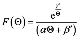 (24)
(24)
Application of the Taylor series expansion at the initial dimensionless time of zero and dimensionless temperature Q = 1 leads to
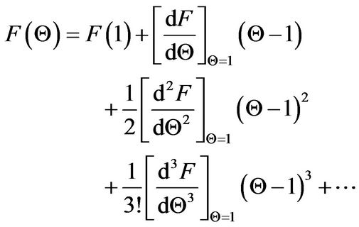 (25)
(25)
The software Mathematica® is used to derive the various derivatives in Equation (25), and the following results were obtained up to the cubic derivative.
 (26)
(26)
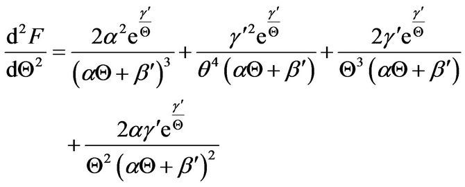 (27)
(27)
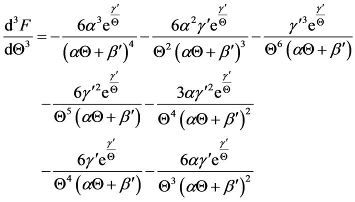 (28)
(28)
In order to understand the F(Q) function, it is plotted in Figure 3 at typical parameter values for both stable and unstable systems, wherein the flat temperature profile is proposed to occur.
From this figure, the area under the curve can be obtained to be equal to the dimensionless time, t. Note that for the stable system, the value of Q approaches infinity at the steady-state value of 5. With the two sets of parameters in Figure 3, the resulting plots of the Dimensionless temperature, Q, vs Dimensionless time, t, is shown in Figure 4.
Since the use of the Exponential Integral function, Ei, as defined in Equation (19), is not well understood in FRRPP systems, comparisons with straight numerical solution and Taylor Series approximations are made and reported in this paper. This exercise is very important for validation of a new conceptual phenomenon that is expressible with a rarely used transcendental function.
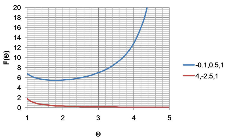
Figure 3. Plots of F(Q) vs Q from Equation (24) for typical sets of parameters representing stable and unstable systems. The legend indicates the triplet of parameters , wherein the stable system represents the set of parameters with negative a.
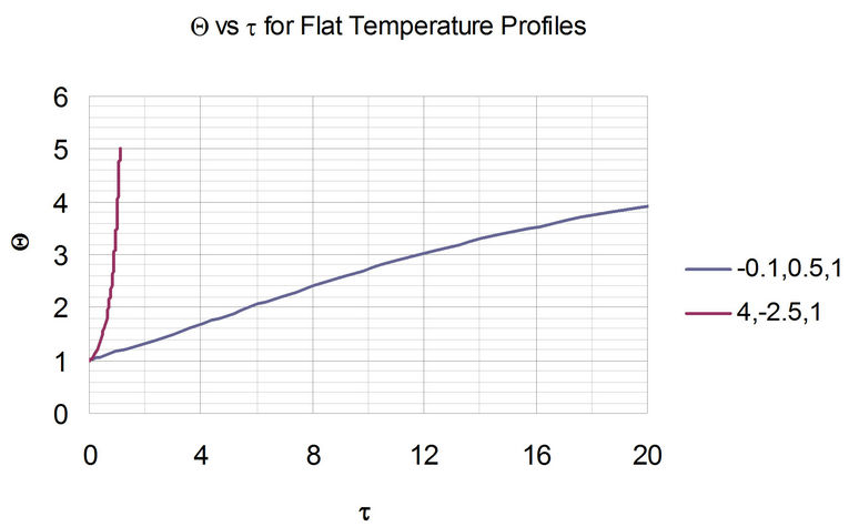
Figure 4. Evolution of flat temperature profile from typical parameter sets for stable and unstable systems. The legend indicates the triplet of parameters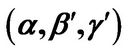 , wherein the stable system represents the set of parameters with negative a. Also, note that as t increases beyond 20, the value of Q asymptotically approaches the steady-state value of 5.
5. Results of Polynomial Approximations
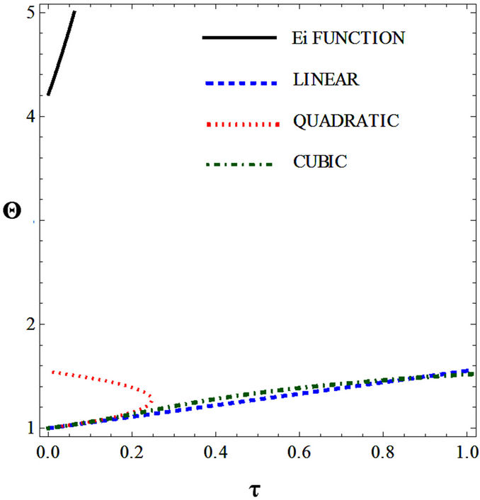
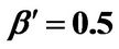
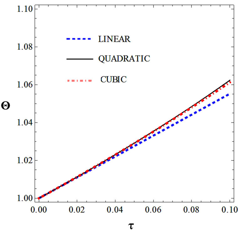
Figures 5(a) and 6(a) show polynomial approximation results of Q vs t for flat temperature profile histories involving typical stable and unstable parameter systems, which could be compared to numerical results in Figure 4. This stable system curve in Figure 4, in turn, has been found to compare very well with Figure 5(b), which is the numerical result of the solution of the full differential equation in Equation (22). For a representative unstable system, the dashed-curve result in Figure 4 is compared with polynomial approximation results in Figure 6(a). This representative unstable system curve in Figure 4, in turn, has been found to compare well with Figure 6(b), which is the numerical result of the solution of the full differential equation in Equation (22). In addition, exponential integral results are shown for given parameter sets in Figures 5(a) and 6(a). Figures 7(a) and 7(b) show expanded abscissa scales for Figures 5(a) and 5(b), for additional comparisons. On the other hand, Figures 8(a) and 8(b) show shorter time behavior for conditions associated with Figures 6(a) and 6(b).
These plots indicate the validity of the use of the numerical approaches, compared to the Ei approximation method using Equation (14). If one uses the polynomial approximation, for a < 0, the linear approximation would be quite accurate in the initial 60% - 70% Q-range, while the cubic approximation would be accurate in the initial 20% Q-range. For a > 0, linear and cubic approximations seem to be accurate in the small-times range, or when Q ® 1. A point of caveat here is that the polynomial approximation does not seem to be asymptotic, until the cubic terms are reached. The final obvious point to be made here is that for a < 0, the analytical-based Ei function is reasonably accurate at the above 20% Q-range.
 (a)
(a)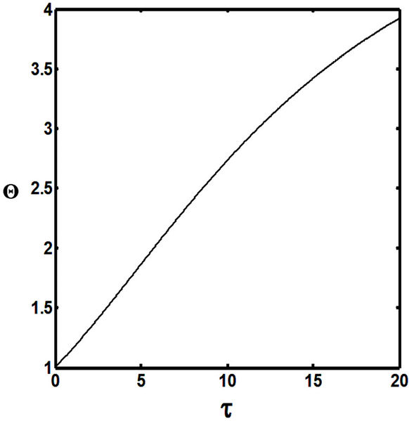 (b)
(b)
Figure 5. (a) Approximation results of Q vs t for flat temperature profile histories involving a typical stable parameter system, represented by ,
,  ,
, ; (b) Numerical results of Q vs t for flat temperature profile histories involving a typical stable parameter system, represented by
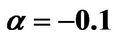 ,
,  ,
, .
.
 (a)
(a) (b)
(b)
Figure 6. (a) Approximation results of Q vs t for flat temperature profile histories involving a typical stable parameter system, represented by ,
,  ,
, ; (b) Numerical results of Q vs t for flat temperature profile histories involving a typical unstable parameter system, represented by
 ,
,  ,
, .
.
6. Conclusion
The quantitative analysis of the occurrence of the flat temperature profile in spherical FRRPP systems indicates that numerical approaches to predict its evolution would be reasonably accurate. If an analytical approximation is to be done, for a < 0, the approach would be to use the linear Taylor series approximation up to 30% - 40% of the Q-range, and continuing to steady-state condition with the use of the Exponential Integral, Ei, function. For a > 0, the only conclusion that can be made is that both linear and cubic polynomial approximations are reasonably accurate at very small times and low Q-values, i.e., at τ → 0 and Q ® 1.
 (a)
(a)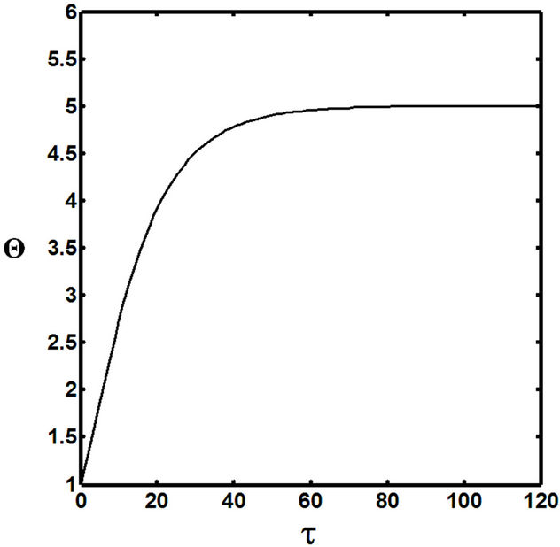 (b)
(b)
Figure 7. (a) Longer abscissa range version of Figure 5(a), for flat temperature profile histories involving a typical stable parameter system, represented by ,
,  ,
, ; (b) Longer abscissa range version of Figure 5(b), for flat temperature profile histories involving a typical stable parameter system, represented by
 ,
,  ,
, .
.
 (a)
(a)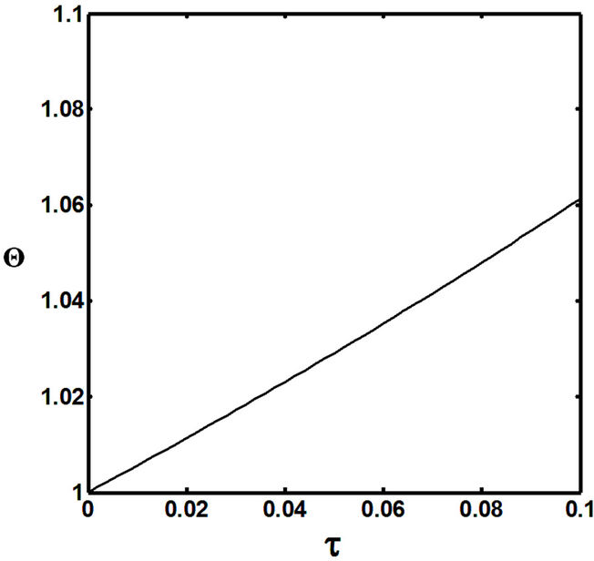 (b)
(b)
Figure 8. (a) Shorter abscissa range version of Figure 6(a), represented by ,
,  ,
, ; (b) Shorter abscissa range version of Figure 6(b), represented by
 ,
,  ,
, .
.
7. Acknowledgements
The authors are grateful for the support of the Michigan Tech Center for Environmentally Benign Functional Materials, the King Abdullah Scholarship Program, Najran and Michigan Tech Universities that allowed the continued work and publication of the quantitative investigation of the FRRPP process.
REFERENCES
- G. T. Caneba, “Free-Radical Retrograde-Precipitation Polymerization (FRRPP): Novel Concept, Processes, Materials, and Energy Aspects,” Springer-Verlag, Heidelberg, 2010.
- G. T. Caneba and Y. L. Dar, “Emulsion Free-Radical Retrograde-Precipitation Polymerization,” Springer-Verlag, Heidelberg, 2011. doi:10.1007/978-3-642-19872-4
- M. A. A. Alharthi, “Dynamic Thermal Behavior of the FreeRadical Retrograde-Precipitation Polymerization (FRRPP) and Related Processes,” M.S. Thesis, Michigan Technological University, Houghton, 2010.
- Y. Dar and G. T. Caneba, “Transport Phenomena Aspects of the Free-Radical Retrograde-Precipitation Polymerization (FRRPP) Process,” Chemical Engineering Communications, Vol. 189, No. 5, 2002, pp. 571-607. doi:10.1080/00986440211745
- B. Wang, Y. Dar, L. Shi and G. T. Caneba, “Polymerization Control Through the Free-Radical Retrograde-Precipitation Polymerization (FRRPP) Process,” Journal of Applied Polymer Science, Vol. 71, No. 5, 1999, pp. 761- 774. doi:10.1002/(SICI)1097-4628(19990131)71:5<761::AID-APP10>3.0.CO;2-S
- G. Odian, “Principles of Polymerization,” John Wiley and Sons, New York, 1991.
- J. Spanier and K. B. Oldham, “An Atlas of Functions,” Hemisphere Publishing Corporation, New York, 1987.
1. Nomenclatures
1.1. Alphabets
1.1.1. Upper Case
A: Defined in Equation (8), dimensionless B: Defined in Equation (9), dimensionless E: Activation energy for reaction, J/mol F: Defined in Equation (24)
R: Universal gas constant, J/mol-K T: Absolute temperature, K X: Defined in Equations (10)-(11), dimensionless
1.1.2. Lower Case
a: Defined in Equation (10)
b: Defined in Equation (10)
k: Thermal conductivity of the reaction fluid r: Radial distance, m or cm
1.2. Subscripts
a: pertains to Activation energy (Equation (5))
M: Pertains to monomer in Equation (11)
P: pertains to polymer in Equation (11)
0: pertains to Pre-exponential rate coefficient (Equations (3),(4),(8),(9)) or Dimensionless Energy Source Term ( Equation (12))
1.3. Superscripts
P: Pertains to polymer-rich phase in Equation (11)
1.4. Greek Symbols
α: Dimensionless version of a from Equation (3)
β: Dimensionless version of b from Equation (4)
γ: Dimensionless activation energy, defined in Equation (5)
η: Dimensionless radius, defined in Equation (7)
ρ: Density, g/cm3 or kg/m3
θ: Dimensionless temperature, defined in Equation (6)
Q: Dimensionless temperature, defined in Equation (16)
t: Dimensionless time, defined in Equation (15)
Φ: Dimensionless heat of polymerization, defined in Equation (2)
1.5. Other Symbols
 : Defined in Equation (12), dimensionless Ei(x): Exponential integral function, defined in Equation (20)
fP: Polymer radical fraction
ΔHP: Heat of polymerization, J/mol ko’: Pre-exponential factor of rate coefficient, defined in Equations (3),(4),(8),(9)
kP: Propagation rate coefficient, Li/mol-s
Φ0: Dimensionless energy source term at the center of the particle, defined in Equation (12)
r0: Particle radius, cm or m XP: Defined in Equation (11)
 : Defined in Equation (11)
 : Defined in Equation (11)