Journal of Mathematical Finance
Vol.2 No.1(2012), Article ID:17599,8 pages DOI:10.4236/jmf.2012.21009
The Distribution of the Value of the Firm and Stochastic Interest Rates
1School of Computer Science, University of Oklahoma, Norman, USA
2Division of Finance, Michael F. Price College of Business, University of Oklahoma, Norman, USA
Email: *dstock@ou.edu
Received September 14, 2011; revised October 4, 2011; accepted October 30, 2011
Keywords: alue of firm; lognormal; interest rate process
ABSTRACT
The time evolution of the value of a firm is commonly modeled by a linear, scalar stochastic differential equation (SDE) of the type 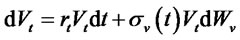 where the coefficient
  in the drift term denotes the (exogenous) stochastic short term interest rate and
  is the given volatility of the value process. In turn, the dynamics of the short term interest rate,
  , are modeled by a scalar SDE. It is shown that
  exhibits a lognormal distribution when
  is a normal/Gaussian process defined by a common variety of narrow sense linear SDEs. The results can be applied to different financial situations where modeling value of the firm is critical. For example, with the context of the structural models, using this result one can readily compute the probability of default of a firm.
1. Introduction
Modeling the value of the firm is one of the more important research topics in finance. The value of an unlevered firm is the value of expected future cash flows discounted at a rate appropriate for an all-equity firm whereas the value of a levered firm is commonly expressed as the value of an unlevered firm plus the gain from leverage due to a tax shield provided by the debt. Including business disruption costs, the optimal capital structure can then be characterized as a trade-off between the interest tax shield and disruption costs. Recent analysis by Hackbarth, Hennessy and Leland [1] extends this line of research by examining an optimal mixture of debt; that is, the optimal mixture of bank debt and market debt (bonds).
Improved models for value of the firm are potentially useful in several contexts. For one example, consider models of credit spreads. Leland and Toft [2] develop an ambitious model of firm value that addresses optimal capital structure, optimal debt maturity, and the term structure of credit spreads. Recently, Qi [3] has modified the Leland and Toft [2] model by setting the lower bankruptcy boundary to be a fraction of bond face value. The importance of good structural models for credit spreads has been enhanced with the growth of credit derivatives and the credit crisis of 2007 and 2008. More specifically, notional amounts of credit derivatives grew by over 100% for every year from 2004 through 2006. At the end of 2006, there was 34.5 trillion outstanding (see Saha-Bubna and Barrett [4]). The weakened credit quality of many financial firms in 2007 and 2008 caused high volatility in equity markets and, also, large changes in the value of credit spreads and credit default swaps.
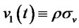
Our purpose is to derive distributions of  whose evolution critically depends on the models for the short term interest rate process,
 . Models for
  can be broadly classified as (a) general linear and (b) non linear models. General linear models are also popularly known as affine models. In this context, we refer to Duffie, Filipovic and Schachermayer [5]; Duffie and Singleton [6]; and Lamberton and Lapeyre [7]. In this paper we are particularly interested in a special class of the general linear models called narrow sense linear models described by Arnold [8].
The next section describes the processes for value of the firm and short term interest rates. Next, we discuss a general framework for the solution of the distribution of . Then, we describe solutions in the cases where
  processes are narrow sense linear. Such
  processes are quite popular for models of credit risk. The shapes of the
  distributions are shown to be sensitive to such parameters as the correlation between the
  and
and  processes. For example, a positive correlation displays a
  distribution with fatter tails than one with negative correlation.
2. The Processes for Value of the Firm and Interest Rates
The time evolution of the value,  , of a firm is routinely modeled under the risk neutral measure by a linear, scalar, stochastic differential equation (SDE)
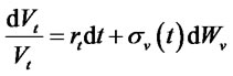 , (1.1)
where the instantaneous drift  denotes the (exogenous) stochastic variable known as the short-term interest rate process and
  is a deterministic function representing the instantaneous volatility as in Acharya and Carpenter [9].
This general form of value process has been used in numerous important structural models of credit risk. For example, see Merton [10] and Acharya and Carpenter [9] where any dividends and coupon payments, outflows of γ from the firm to investors, are subtracted from the rt drift term. Many firms do not pay dividends and our model is one of zero coupon debt so that a γ of zero is reasonable. We note that Longstaff and Schwartz [11] similarly have a zero γ.
The  drift of
  indicates our model is risk neutral. We could assume different firms have different drifts due to such things as different expected returns in their industry as well as different riskiness of assets and future projects. However, such an assumption is arbitrary and yields a model that is not arbitrage free. We believe it is much more theoretically credible to posit a risk neutral, arbitrage free model.
The dynamics of the short term interest rate are modeled, under the same risk neutral measure, by a (scalar) SDE of the type
 , (1.2)
where the instantaneous drift,  and the volatility,
  are smooth functions. It is further assumed that the Wiener increment processes
 ![]() and
and ![]() are correlated; that is,
are correlated; that is,
 (1.3)
(1.3)
with . It is worth noting that in this set up the flow of information is only one way –
 affects
  and not vice versa. By combining several well known results from the literature, in this paper we characterize the distribution of the value process
  for different choices of the
  processes.
All the known stochastic interest rate models can be broadly classified into two classes—single factor models (SFMs) and multi-factor models (MFMs). We refer to Cairns [12] and Privault [13] for details. In this paper, we are primarily interested in the SFMs. These SFMs can be divided into linear and nonlinear models. Following Arnold [8], linear models can be further subdivided into two subclasses. The SFM in (1.2) is called a narrow sense linear model if
 , (1.4)
and
 . (1.5)
A general linear model, on the other hand, has  in the form (1.4) and
 , (1.6)
where and
and  are smooth functions of time
 . The general linear models are also known as affine models as in Duffie, Filipovic, and Schachermayer [5]; Duffie and Singleton [6]; and Lamberton and Lapeyre [7]. The SFM in (1.2) is called a nonlinear model if either
  and/or
  are nonlinear functions of the short rate
 .
.
Refer to Tables 1(a)-(c) for examples of these models. The narrow sense linear models of Merton [14], Vasicek [15], Ho and Lee [16], and Hull and White [17] are special cases of the Heath, Jarrow and Morton [18] model and define normal/Gaussian processes.
We first solve the scalar SDE (1.2) for , and using it in (1.1), we then recover
 . It is well known that
  is a lognormal process when
  a constant. See Kloeden and Platen [19]. We extend this result by first showing that
  also inherits this lognormal distribution where
  is a normal process defined by the narrow sense linear models in Table 1.
This problem of quantifying the probability distribution of  is critical to credit risk analysis. For a review of various approaches to credit risk refer to the books by Duffie and Singleton [6], Bielecki and Rutkowski [20], and Jarrow et al. [21]. Clearly computation of the default probability in structural models requires knowledge of the probability distribution of
  contingent on the chosen model for the interest rate.
3. A framework for the Solution
In this section we develop a framework for solving (1.1)- (1.2). Setting  and applying Ito’s lemma, equation (1.1) becomes.
 . (2.1)
See Kloeden and Platen [19].
Setting  and
and
![]()
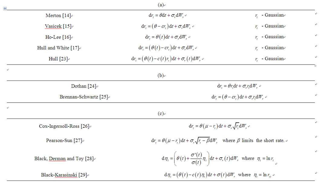
Table 1. Alternative Models of . The single factor model in (1.2) is called a narrow sense linear model if
  and
and . In contrast, the model is called an affine model or a general linear model if
  is of the above form and
 . The model is called nonlinear if either
  and/or
  are nonlinear functions of the short rate
 . (a) Narrow sense linear models; (b) General linear or affine models; (c) Nonlinear models.
(Shreve [22]) we can rewrite the pair of equations (1.2) and (2.1) as
 (2.2)
(2.2)
and
 (2.3)
(2.3)
where  and
and  are two independent Wiener increment processes and
![]() . (2.4)
. (2.4)
Integrating (2.3), we obtain
 (2.5)
(2.5)
where
 (2.6)
(2.6)
and
 . (2.7)
From the properties of the Ito integral, Mikosch [30] and Shreve [22], it follows that
 (2.8)
(2.8)
where
 . (2.9)
Since  and
and  are independent Wiener processes, it readily follows that
  . Thus, the distribution of
  and hence of
  critically depend on the properties of the
  process in (2.2).
In closing this section consider the special case when , a constant. Then,
 . (2.10)
Further, when , we obtain
 . (2.11)
4. Narrow Sense Linear Models for rt
Setting
 , (3.1)
in (2.2), we get a narrow sense (time varying) linear model known as the generalized Hull and White [17] model given by
 . (3.2)
Since all the other narrow sense linear models in Table 1 are special cases of (3.2), we first concentrate on solving (3.2). Defining
 , (3.3)
we get
 . (3.4)
T
his is known as the fundamental solution of (3.2). Hence the solution of (3.2) is given by (Arnold [8], Gard [31], Kuo [32], Lamberton and Lapeyre [7]) , (3.5)
where
 , (3.6)
 , (3.7)
and
 . (3.8)
Hence,
 (3.9)
(3.9)
where
 . (3.10)
Now combining (3.5)-(3.10), it follows that
 . (3.11)
Applying integration by parts to the second integral on the right hand side of (3.11) and using (3.7), it follows that
 (3.12)
Is also a Gaussian process with mean zero and variance given by
 . (3.13)
Substituting (3.11)-(3.12) in (2.5), we get
 (3.14)
where
 (3.15)
and
 . (3.16)
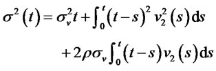
Substituting (2.6), (3.12) and (2.7) in (3.16), the latter becomes
 (3.17)
Since  and
and  are independent, it follows that
  where
where
 (3.18)
 , (3.19)
where

and
 .
.
Combining (3.15)-(3.18) with (3.14), we finally obtain
 (3.20)
where given by (3.16) and
  given by (3.19).
We summarize the above developments in the following:
Theorem 3.1: Let the interest rate  evolve according to a narrow sense linear, scalar, SDE of the type (3.2). Then,
  is a Gaussian process and consequently
  in (2.5) is also a Gaussian process given by (3.20).
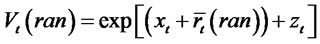
Since , from (3.14)-(3.20), we get
 (3.21)
where
 (3.22)
and
 . (3.23)
The following corollary is immediate.
Corollary 3.2: Since ,
,
 is a lognormal process whose probability density function, as a function of time, is given by
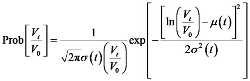 . (3.24)
It can be verified (Johnson et al. [33]) that the time evolution of the mean and variance of the value process
 are given by
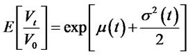 (3.25)
and
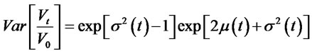 . (3.26)
We now enlist a number of nested corollaries by considering special cases of interest rate models.
Case 1: Let , a constant. Then
 ,
, ![]() and
and  is given by
(3.8). From (3.15) and (3.20), the mean is
 (3.27)
where  is given in (3.6). From (3.19)-(3.20), the variance is
 . (3.28)
Case 2: Hull and White [17] model: In this model,  and
and  where
where  and
and  are constants. Thus,
  ,
,  and
and
 . (3.29)
Hence the mean is
(3.30)
and the variance is
 (3.30a)
 . (3.30b)
Case 3: Ho-Lee [16] model: In this model,  and
and . Then
 . (3.31)
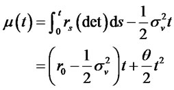
The mean is
 (3.32)
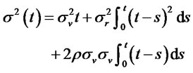
and the variance is
 (3.33a)
 . (3.33b)
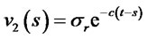
Case 4: Vasicek [15] model: In this model,  ,
,  and
and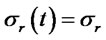 . Then,
  and
and
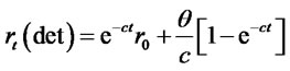 . (3.34)
Hence, the mean is
 (3.35a)
 (3.35b)
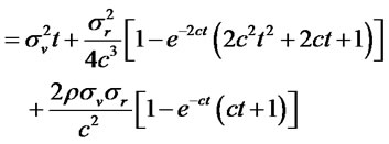
and the variance is
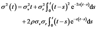 (3.36a)
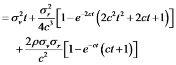 . (3.36b)
Case 5: Merton [14]: In this case,  ,
,  and
and . Then
  and
and
 . (3.37)
Hence, the mean is
 (3.38)
and the variance is
 (3.39a)
 . (3.39b)
C
ase 6: Let , a constant and
 . Then
 ,
,  and
and . The mean
 (3.40)
and the variance
 . (3.41)
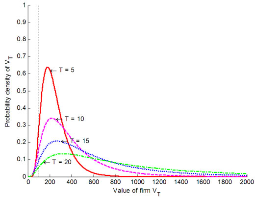
We now provide sample plots of the  distribution, when
  follows the Vasicek [15] model, for three different values of the correlation (
 , 0.9 and −0.9) in Figures 1-3 respectively. In each case the distribution of
  for
for 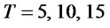 and 20 are given. From these figures it follows that as
 ![]() increases both the mean and variance of
increases both the mean and variance of  increases. Further, comparing Figures 1 and 2, it follows that the effect of the positive correlation (
 ) is to reduce the peak while making the tails fatter compared to the case when
 . Similarly from Figures 1 and 3, we readily see the negative correlation has the opposite effect of increased peak and thinner tails compared to
 .
.
The primary motivation for characterizing the distribution of  is to compute the probability of default. Within the framework of structural models, there has been an evolution of the definition of default. In the now classic paper, Merton [10] defines default as the event
 ![]() bond with maturity
bond with maturity![]() . Using the results described above, we could readily compute the probability default according to this classical definition1.
. Using the results described above, we could readily compute the probability default according to this classical definition1.
 for Vasicek with
 ,
,  ,
,  ,
,  ,
,  ,
,  ,
,

 for Vasicek with
 ,
,  ,
,  ,
,  ,
,  ,
,  ,
,

 for Vasicek with
 ,
,  ,
,  ,
,  ,
,  ,
,  ,
,
However, Longstaff and Schwartz [11] define default by the event . Recently, Giesecke [34] has expanded on this theme and has defined the default by the compound event
  for
for .
.
Recall that the probability of these later events can be readily calculated using the “reflection principle” if  is a standard Wiener process or by using the Girsanov theorem if
  is a Wiener process with a drift. (See Elliott and Kopp [35] and Giesecke [34]). To enable computation of default probability according to Giesecke [34], in the following, we seek to express
  in (3.14) as the sum of a drift term and a (time changed) Wiener process.
To this end recall that every Ito integral is equivalent to a time changed Wiener process. (See Shiryaev [36], Oksendal [37], Karatzas and Shreve [25]). Accordingly, from (3.17) we obtain
 (3.42)
where  and
and  are two independent Wiener process with
 ,
,
and  and
and  are given in (3.19). Since
  and
and  are independent, there exists a Wiener process
  such that
 (3.43)
where
as given by (3.18)-(3.19).
Combining (3.43) with (3.14), it follows that
 (3.44)
where  as in (3.20).
5. Conclusions
We have analyzed the impact of  on
on  when
when  evolves according to a narrow sense linear model in Table 1(a). Consider the case when
  evolves according to a general linear model, such as for example, the Brennan-Schwartz [38] model in Table 1(b). In this case the explicit form of the solution for
  is well known (Arnold [8], Gard [15], Lamberton and Lapeyre [7]) and is given by

where the process  is given by
 with
with . Hence,
 involves a process
which is an integral of the exponential functionals of the Wiener process. Processes of the type  routinely arise in the evaluation of Asian type options (Vorst [39]). By relating
  to a Bessel process, Yor [40] and Geman and Yor [41] have provided a complete characterization of the distribution of the
  process. Combining these results with (2.5) to derive the distribution of
  is an interesting open problem. Similarly, computing the distribution
  when
when  evolves according to the nonlinear models is Table 1(c) is also wide open. Solutions to these problem will shed further light on the impact of the choice of interest rate models on default probability and hence on credit risk analysis.
6. Acknowledgements
We are grateful to Robert J. Elliott (University of Calgary) and to Luciano Campi (Universite Paris Dauphine) for their interest and comments that improved the presentation.
REFERENCES
- D. Hackbarth, C. A. Hennessy and H. E. Leland, “Can the Trade-Off Theory Explain Debt Structure?” Review of Financial Studies, Vol. 20, No. 1, 2007, pp. 1389-1428. doi:10.1093/revfin/hhl047
- H. E. Leland and K. B. Toft, “Optimal Capital Structure, Endogenous Bankruptcy, and the Term Structure of Credit Spreads,” Journal of Finance, Vol. 51, No. 3, 1996, pp. 987-1019. doi:10.2307/2329229
- H. Qi, “Credit Spread by a Modified Leland-Toft Model,” FMA Meetings, Orlando, 18-20 October 2007, unpublished.
- A. Saha-Bubna and E. Barrett, “Credit Derivatives Show Surge,” Wall Street Journal, Vol. 255, No. 98, 2007, p. c1.
- D. Duffie, D. Filipovic and W. Schachermayer, “Affine Processes and Applications in Finance,” The Annals of Probability, Vol. 13, No. 3, 2003, pp. 984-1053. doi:10.1214/aoap/1060202833
- D. Duffie and K. J. Singleton, “Credit Risk: Pricing, Measurement, and Management,” Princeton University Press, Princeton, 2003.
- D. Lamberton and B. Lapeyre, “Introduction to Stochastic Calculus applied to Finance,” English Edition, Translated by N. Rabeau and F. Mantion, 2nd Edition, Chapman & Hall, London, 2007.
- L. Arnold, “Stochastic Differential Equations: Theory and Applications,” John Wiley & Sons, New York, 1974.
- V. V. Acharya and J. N. Carpenter, “Corporate Bond Valuation and Hedging with Stochastic Interest Rate and Endogenous Bankruptcy,” The Review of Financial Studies, Vol. 15, No. 5, 2002, pp. 1355-1383. doi:10.1093/rfs/15.5.1355
- R. C. Merton, “On the Pricing of Corporate Debt: The Risk Structure of Interest Rates,” Journal of Finance, Vol. 29, No. 3, 1974, pp. 449-470. doi:10.2307/2978814
- F. A. Longstaff and E. S. Schwartz, “A Simple Approach to Valuing Risky Fixed and Floating Rate Debt,” Journal of Finance, Vol. 50, No. 3, 1995, pp. 789-819. doi:10.2307/2329288
- A. J. G. Cairns, “Interest Rate Models: An Introduction,” Princeton University Press, Princeton, 2004.
- N. Privault, “An Elementary Introduction to Stochastic Interest Rate Modeling,” World Scientific, Singapore, 2008.
- R. C. Merton, “Theory of Rational Option Pricing,” Bell Journal of Economics and Management Science, Vol. 4, No. 1, 1973, pp. 141-183. doi:10.2307/3003143
- O. Vasicek, “An Equilibrium Characterization of the Term Structure,” Journal of Financial Economics, Vol. 37, 1977, pp. 339-348.
- S. Y. Ho and S. B. Lee, “Term Structure Movements and Pricing Interest Rate Contingent Claims,” Journal of Finance, Vol. 41, No. 5, 1986, pp. 1011-1029. doi:10.2307/2328161
- J. C. Hull and A. D. White, “Pricing Interest Rate Derivative Securities,” Review of Financial Studies, Vol. 3, No. 4, 1990, pp. 573-592. doi:10.1093/rfs/3.4.573
- D. Heath, R. Jarrow and A. Morton, “Bond Pricing and Term Structure of Interest Rates: A New Methodology for Contingent Claims Valuation,” Econometrica, Vol. 60, No. 1, 1992, pp. 77-105. doi:10.2307/2951677
- P. E. Kloeden and E. Platen, “Numerical Solution of Stochastic Differential Equations,” Springer-Verlag, New York, 1992.
- D. R. Bielecki and M. Rutkowski, “Credit Risk: Modeling, Valuation and Hedging,” Springer, New York, 2002.
- R. A. Jarrow, D. Lando and S. M. Turnbull, “A Markov Model for the Term Structure of Credit Risk Spreads,” Review of Financial Studies, Vol. 10, No. 2, 1997, pp. 481-523. doi:10.1093/rfs/10.2.481
- S. E. Shreve, “Stochastic Calculus Models for Finance,” Springer, New York, 2004.
- J. C. Hull, “Options, Futures and other Derivatives,” 4th Edition, Prentice Hall, Englewood Cliff, 2000.
- M. U. Dothan, “On the Term Structure of Interest Rates,” Journal of Financial Economics, Vol. 62, No. 6, 1978, pp. 59-69. doi:10.1016/0304-405X(78)90020-X
- J. Cox, J. Ingersoll and S. Ross, “A Theory of the Term Structure of Interest Rates,” Econometrica, Vol. 53,
- I. Karatzas and S. E. Shreve, “Brownian Motion and Stochastic Calculus,” Springer-Verlag, New York, 1991. doi:10.1007/978-1-4612-0949-2
- No. 2, 1985, pp. 385-407. doi:10.2307/1911242
- N. Pearson and T. S. Sun, “An Empirical Examination of the Cox-Ingersoll-Ross Model of Term Structure of Interest Rates Using the Method Maximum Likelihood,” Journal of Finance, Vol. 54, 1994, pp. 929-959.
- F. Black, E. Derman and W. Toy, “A One-factor Model of Interest Rates and Its Application to Treasury Bond Options,” Financial Analyst’s Journal, Vol. 46, No. 1, 1990, pp. 33-39. doi:10.2469/faj.v46.n1.33
- F. Black and P. Karasinski, “Bond and Option Pricing When Short Rates Are Log-Normal,” Financial Analysis Journal, Vol. 47, No. 4, 1991, pp. 52-59. doi:10.2469/faj.v47.n4.52
- T. Mikosch, “Elementary Stochastic Calculus with Finance in View,” World Scientific, Singapore, 1999.
- T. C. Gard, “Introduction to Stochastic Differential Equations,” Marcel Dekker Inc., New York, 1988.
- H. H. Kuo, “Introduction to Stochastic Integration,” Springer, New York, 2006.
- N. L. Johnson, S. Kotz and N. Balakrishnan, “Continuous Univariate Distributions,” 2nd Edition, John Wiley & Sons, Inc., New York, 1994.
- K. Giesecke, “Credit Risk Modeling and Valuation: An Introduction,” In: D. Shimko, Ed., Credit Risk: Models and Management, Riskbooks, London, 2004, pp. 1-67.
- R. Elliott and P. Kopp, “Mathematics of Financial Markets,” 2nd Edition, Springer-Verlag, New York, 2005
- A. N. Shiryaev, “Essentials of Stochastic Finance: Facts, Models, Theory,” World Scientific, New York, 1999. doi:10.1142/9789812385192
- B. Oksendal, “Stochastic Differential Equations: An Introduction with Applications,” 6th Edition, Springer Verlag, New York, 2003.
- M. Brennan and E. Schwartz, “A Continuous-Time Approach to the Pricing of Bonds,” Journal of Banking and Finance, Vol. 3, No. 4, 1979, pp. 133-155. doi:10.1016/0378-4266(79)90011-6
- T. Vorst, “Prices and Hedge Ratios of Average Exchange Rate Options,” International Review of Financial Analysis, Vol. 1, No. 3, 1992, pp. 179-193. doi:10.1016/1057-5219(92)90003-M
- M. Yor, “On Some Exponential Functionals of Brownian Motion,” Advances in Applied Probability, Vol. 24, No. 3, 1992, pp. 509-531. doi:10.2307/1427477
- H. Geman and M. Yor, “Bessel Processes, Asian Options, and Perpetuities,” Mathematical Finance, Vol. 3, No. 4, 1993, pp. 349-375. doi:10.1111/j.1467-9965.1993.tb00092.x
- D. C. Shimko, N. Tejima and D. Van Deventer, “The Pricing of Risky Debt When Interest Rates Are Stochastic,” Journal of Fixed Income, Vol. 3, No. 2, 1993, pp. 58- 65. doi:10.3905/jfi.1993.408084
NOTES
*
Corresponding author.1
We note that Shimko, Tejima, and Van Deventer [42] build upon the Merton [11] model and solve for bond and equity prices as opposed to value of the firm.