Open Journal of Statistics
Vol.07 No.04(2017), Article ID:78344,18 pages
10.4236/ojs.2017.74045
Generalized Inverted Kumaraswamy Distribution: Properties and Application
Zafar Iqbal1*, Muhammad Maqsood Tahir1, Naureen Riaz2, Syed Azeem Ali3, Munir Ahmad4
1Department of Statistics, Government College, Gujranwala, Pakistan
2Garrison University, Lahore, Pakistan
3Department of Statistics, Government College, Lahore, Pakistan
4National College of Business Administration and Economics, Lahore, Pakistan

Copyright © 2017 by authors and Scientific Research Publishing Inc.
This work is licensed under the Creative Commons Attribution International License (CC BY 4.0).
http://creativecommons.org/licenses/by/4.0/


Received: June 17, 2017; Accepted: August 8, 2017; Published: August 11, 2017
ABSTRACT
The techniques to find appropriate new models for data sets are very popular nowadays among the researchers of this area where existed models in the literature are not suitable. In this paper, a new distribution, generalized inverted Kumaraswamy (GIKum) distribution is introduced. The main aims of this research are to develop a general form of inverted Kumaraswamy (IKum) distribution which is flexible than the IKum distribution and all of its related and sub models. Some properties of GIKum distribution such as measures of central tendency and dispersion, models of stress-strength, limiting distributions, characterization of GIKum distribution and related probability distributions through some specific transformations are derived. The mathematical expressions of reliability function (r.f) and the hazard rate function (hrf) of the GIKum distribution are found and presented through their graphs. The parameters estimation through the maximum likelihood (ML) estimation method is used and the results are applied to the data set of prices of wooden toys of 31 children.
Keywords:
Generalized Inverted Kumaraswamy Distribution, Stress-Strength Models, Maximum Likelihood Estimation

1. Introduction
In the past years, several ways of generating inverted distributions from classic ones were developed and discussed. Calabria and Pulcini [1] defined the inverse Weibull distribution. AL-Dayian [2] introduced a family of distributions that arises naturally from the inverted Burr type XII distribution. Abed El-Kader et al. [3] proposed the inverted Pareto type I distribution and introduced some properties of this class of distributions.
A number of researchers studied the inverted distributions and its applications; for example, Prakash [4] studied the inverted exponential model and Aljuaid [5] presented exponentiated inverted Weibull distribution. The inverted distributions are important in problems related to econometrics, engineering sciences, life testing, financial literature and environmental studies.
Kumaraswamy [6] obtained a distribution, which is derived from beta distribution after fixing some parameters in beta distribution. But it has a closed-form cumulative distribution function which is invertible and for which the moments do exist. The distribution is appropriate to natural phenomena whose outcomes are bounded from both sides, such as the individuals’ heights, test scores, temperatures and hydrological daily data of rain fall (for more details, see Kumaraswamy [6] , Jones [7] , Golizadeh et al. [8] , Sindhu et al. [9] and Sharaf El-Deen et al. [10] ).
Abd Al-Fattah et al. [11] derived the inverted Kumaraswamy (IKum) distribution from Kumaraswamy (Kum) distribution using the transformation . When where and are shape parameters, then the has a IKum distribution with probability density function (pdf)
(1)
Iqbal et al. generalized the some continuous distribution by using power transformation. Here we use the same technique to find the cdf of generalized inverted Kumaraswamy distribution (GIKum) and is derived by using transformation which has closed form and is as under
(2)
Assuming X is a random variable with shape parameters, , and the pdf of GIKum is as
#Math_13# (3)
This model is flexible enough to accommodate both monotonic as well as non-monotonic failure rates.
From Figure 1, the GIKum pdf is positively skewed distribution for all parameters’ values and for , the GIKum pdf is monotonically decreasing. The asymptote of distribution occurs at and is . The GIKum pdf has the higher peaked for larger when other parameters values are fixed.
This paper is arranged as follows. In Section 2, some statistical properties of GIKum distribution such as measures of central tendency and dispersion, reliability function (rf) hazard rate functions (hrf) and reverse hazard function, models of stress-strength, mode, moment generating function, the asymptotic mean and variance, incomplete moments, quantile functions, mean deviation and

Figure 1. PDF of the GIKum distribution for different parameter values.
Renyi entropy are analyzed [12] . In Section 3, sub-models and limiting distributions of GIKum and the related probability distributions of GIKum are derived through some specific transformations. In Section 4, characterization of GIKum is presented. In Section 5, maximum likelihood estimation for the parameters is obtained with some useful remarks and a theorem. Finally, in Section 6, we have applied this on real data set of prices of wooden toys of 31 children.
2. The Main Properties of the Generalized Inverted Kumaraswamy Distribution
This section is devoted to illustrate some statistical properties of GIKum distribution, through rf, some models of the stress-strength, hrf and reversed hazard (rhrf), measures of central tendency and dispersion, graphical and order statistics (Figure 2).
2.1. Reliability Function
(4)

Figure 2. Survival function of the GIKum distribution for different parameter values.
2.2. Hazard Function and Reverse Hazard Function of GIKum Distribution (Figure 3 & Figure 4)
Suppose if the distribution function is defined as
then [2] written as
The hazard rate function (hrf) denoted by and reverse hrf denoted by are given, respectively, by
and
and their relations are shown as under
where
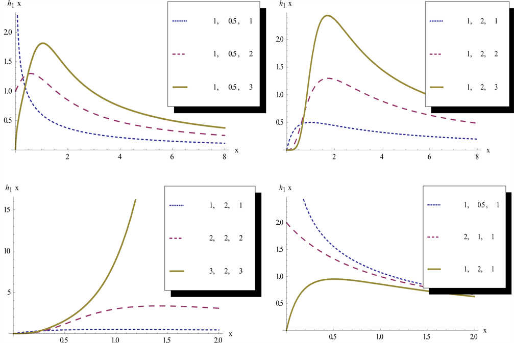
Figure 3. Hazard rate function of the GIKum distribution for different parameter values.

Figure 4. Reverse hazard rate function of the GIKum distribution for different parameter values.
For
For .
and relation in reverse hrf of F and G as and cdf can be expressed as
.
2.3. Some Stress-Strength Models
1) Let T be the stress component subject strength Y, the random variables T and Y are independent distributions from GIKum (α, β, γ) respectively, then the reliability function is given by;
Let T and Z be two independent random stress variables with known cdfs (𝑡), 𝐺(𝑧), and both follow and respectively, and let Y be, independent of T and Z, a random strength variable follow to
2.4. The Mode of the Generalized Inverted Kumaraswamy Distribution
The mode of the GIKum distribution is given by
When ,
The mode of the GIKum distribution is given by
When ,
2.5. Quantiles of the Generalized Inverted Kumaraswamy Distribution
The quantile function of the GIKum is given by
Special cases can be obtained using [10] such as the second quartile (median), when q = 0.5
2.6. The Central and Non-Central Moments
The rth non central moment of the GIKum (α, β) distribution is given by
where is the beta function.
The central moments can be obtained by applying the general relation in central and the non-central moments which as follows
Thus the mean and variance of GIKum when are given by
,
and
The Asymptotic Mean and Variance
If with and then the variable
. This relation can be used to approximate the mean and variance
where
2.7. Moments and Moment Generating Function
where is defined as
2.8. Quantile Functions
2.9. Incomplete Moments
The rth incomplete moments of GIKum distribution is
where
2.10. Mean Deviation
The mean deviation of GIKum
2.11. Rényi Entropy
The Rényi entropy of an r.v X is defined as
where , and using the pdf of GIKum
expanding the last term of integrand through binomial expansion which simplifies as
Again, applying the same expansion we have
Using the transformation in above expression and simplifying,
the Rényi entropy, hence, finally reduces to
3. Related Distributions
This section discussed some sub-models of GIKum distribution, some relations of the GIKum distribution to other distributions, limiting and several IKum G families of distributions.
3.1. Some Sub-Models
3.1.1. Lomax (Pareto Type II) Distribution
The Lomax (Pareto type II) distribution is a special case from GIKum distribution, when in (2) with the following pdf
3.1.2. Beta Type II (Inverted Beta) Distribution
The inverted beta type II (β, 1) is a special case from GIKum distribution, when in (2)
Also when then
3.1.3. The Log-Logistic (Fisk) Distribution
The log-logistic (Fisk) distribution is a special case from IKum distribution, when in (2), with the following form
3.2. Some Relations between the Inverted Kumaraswamy Distribution and Other Distributions
The inverted distribution can be transformed to several distributions using appropriate transformations such as exponentiated Weibull (exponentiated exponential, Weibull, Burr type X, exponential, Rayleigh), generalized uniform (beta type I, inverted generalized Pareto type I, uniform (0, 1)), left truncated exponentiated exponential (left truncated exponential, exponential), exponentiated Burr type XII (Burr type XII, generalized Lomax, beta type II, F- distribution), Kumaraswamy-Dagum (Dagum, Kumaraswamy-Burr type III, Burr type III, log logistic) and Kumaraswamy-inverse Weibull (Kumaraswamy-inverse exponential, inverse exponential). Table 1 summarizes the transformations from IKum to other distributions.
Limiting Distributions
1) If and on then the PDF of y is

Table 1. Values of Mode for different values of and when .
If then it is the pdf of the inverted Weibull distribution.
2) If and then the pdf of y is and as the pdf of y tends to , which is the pdf of the generalized exponential distribution.
3) If and on , then the pdf of y is As
both and the pdf of y tends to which is the pdf of the standard extreme value distribution of the first type (Table 2).
4. Characterizations Based on Conditional Expectation
Characterization of a probability distribution for continuous r.v is important in several research areas and has recently involved many researchers attention. Here we characterize generalized inverted Kumaraswamy distribution based on 1) relationship of two moments based on truncation; 2) truncated moments of the statistic of nth order with certain functions.
4.1. Characterizations Based on Two Truncated Moments
Following Hamedani [13] , we are going to mention here that the advantage of this characterization is twofold: it relates the cdf or pdf of a distribution to the solution of the differential equation of a first order type and further there is not necessary for simple format of cdf.
Theorem 4.1
Let probability space and for a < b with and ,
Table 2. Summary of some transformations applied to the generalized inverted Kumaraswamy and the resulting distribution.
where as the interval H is defined as H = [a, b]. Suppose continuous r.v X with cdf F where X is such that and let both g, h be functions of real type on H satisfying the following expression
where is a real function. Furthermore, assuming that g, are continuous and F are differentiable twicely and F monotone function on H. Finally, assuming the equation and it has never any solution in real belongs to H. and then F is determined uniquely from the following relation
and the function has a solution of and C is chosen so that .
The condition in which the both functions and are integrable uniformly and the cdf relatively compact form, and in distribution if
Proposition 4.1
Let be an r.v and let and . The pdf of X is (2) if defined in 2.1 theorem and has the following form for .
Proof. Let X has density (1.3), then
and and finally for
Conversely, when is defined earlier, then
and finally hence
Now, from 2.1 theorem, X has pdf (3)
Corollary 4.1
Let be an r.v with proposition in 4.1. The pdf of X is (2) if there exist and functions given in 4.1 theorem with the following differential equation (DE)
Remark 4.1. (a) The DE has the general solution of 4.1 corollary of the form
for , where a new constant D is introduced and it may be in particular value according to proposition 4.1.
4.2. Characterization through the Statistic of nth Ordered Truncated Moment
This section contains the characterizations of GIKum distribution based on function of the last order statistics. This characterization is derived through the consequence of the proposition 4.2, which is similar to the Hamedani [13] .
Proposition 4.2
Let be a r.v with cdf F. let and be two differentiable functions on such that and
Then
implies
Taking, e.g. and , will be a result in (2).
5. Maximum Likelihood (ML) Estimators of GIKum Distribution’s Parameters
We present here a ML estimator of the parameters of GIKum distribution
(5)
and
(6)
Taking partial derivatives with respect to and respectively from (6), we have
(7)
(8)
(9)
The ML estimators say of , are found through solution of the nonlinear system. This system of nonlinear equations does not provide explicit functions of the estimators of the parameters of GIKum distribution. Therefore, for the solution of this system of equations using software can be estimated numerically with R.
For the inference about model parameters i.e. the point estimation and the testing of hypothesis we require the information matrix of order 3 × 3 which have partial derivatives of second order and they derived from Equations (7)-(9) with again differentiating. Assuming that the regularity conditions holds, the vector follows the multivariate normal distribution asymptotically i.e. , where and is an information matrix.
We conclude this section by expressing in terms of a random variable whose distribution will be derived in the next section.
where
5.1. Distributions of and
The following remarks and a theorem illustrate the distributions of and .
5.1.1. Remarks
The following conclusions can be obtained easily which we present them as remarks.
i) If with known, then follows .
ii)
iii)
iv) In view of (2), .
v) If are i.i.d. Gamma (β, n), then the ith transformed ordered failures are i.i.d. Exp(β).
vi)
5.1.2. Moments of
The rth moment of the statistic is
and that of is
Theorem 5.1
Let be i.i.d. random variable with cdf F and let be the nth order statistic. Consider the sequence of random variables The limiting function of is for and .
Proof:
The pdf of is
Let
Differentiating it w.r.t , we have
The pdf of is and its cdf is
Letting , we arrive at and
6. Applications of GIKum Distribution
In this section, the proposed distribution is fitted to the data set of prices of wooden toys of 31 children in April 1991 at Suffolk craft shop (Table 3):
 The maximum likelihood estimates of unknown parameters of GIKUM, Lomax and Beta type-II distributions,
and information criteria are given in Table 4.As the values of
, AIC, BIC and HQIC are smaller for GIKum distribution as compare to Lomax distribution and Beta type-II distribution, GIKumTable 3. Descriptive statistics.table_table_tableTable 4. Maximum likelihood estimates and information criteria.table_table_table
The maximum likelihood estimates of unknown parameters of GIKUM, Lomax and Beta type-II distributions,
and information criteria are given in Table 4.As the values of
, AIC, BIC and HQIC are smaller for GIKum distribution as compare to Lomax distribution and Beta type-II distribution, GIKumTable 3. Descriptive statistics.table_table_tableTable 4. Maximum likelihood estimates and information criteria.table_table_table

Figure 5. Empirical histogram and fitted distributions.
distribution fits better for given data set. The same thing can be confirmed after seeing Figure 5.
7. Concluding Remarks
In this paper, a new distribution called GIKum distribution is introduced. Some properties of GIKum distribution such as measures of central tendency and dispersion, models of stress-strength, limiting distributions, characterization of GIKum distribution and related probability distributions through some specific transformations are derived. The mathematical expressions of reliability function (r.f) and the hazard rate function (hrf) of the GIKum distribution are found and presented through their graphs. The parameters estimation through the technique of maximum likelihood estimation is used and the results are applied to the data set of prices of wooden toys of 31 children.
Cite this paper
Iqbal, Z., Tahir, M.M., Riaz, N., Ali, S.A. and Ahmad, M. (2017) Generalized Inverted Kumaraswamy Distribution: Properties and Application. Open Journal of Statistics, 7, 645-662. https://doi.org/10.4236/ojs.2017.74045
References
- 1. Calabria, R. and Pulcini, G. (1990) On the Maximum Likelihood and Least Squares Estimation in the Inverse Weibull Distribution. Journal of Statistica Applicate, 2, 3-66.
- 2. AL-Dayian, G.R. (1999) Burr Type III Distribution: Properties and Estimation. The Egyption Statistical Journal, 43, 102-116.
- 3. Abd EL-Kader, R.E, AL-Dayian, G.R. and AL-Gendy, S.A. (2003) Inverted Pareto Type I Distribution: Properties and Estimation. Journal of Faculty of Commerce AL-Azhar University, Girls’ Branch, 21, 19-40.
- 4. Prakash, G. (2012) Inverted Exponential Distribution under a Bayesian View Point. Journal of Modern Applied Statistical Methods, 11, 190-202.
https://doi.org/10.22237/jmasm/1335845700 - 5. Aljuaid, A. (2013) Estimating the Parameters of an Exponentiated Inverted Weibull Distribution under Type II Censoring. Journal of Applied Mathematical Sciences, 7, 1721-1736.
https://doi.org/10.12988/ams.2013.13158 - 6. Kumaraswamy, P. (1980) A Generalized Probability Density Function for Double-Bounded Random Processes. Journal of Hydrology, 46, 79-88.
- 7. Jones, M.C. (2009) Kumaraswamy’s Distribution: A Beta-Type Distribution with Some Tractability Advantages. Statistical Methodology, 6, 70-81.
- 8. Golizadeh, A., Sherazi, M.A. and Moslamanzadeh, S. (2011) Classical and Bayesian Estimation on Kumaraswamy Distribution Using Grouped and Ungrouped Data under Difference of Loss Functions. Journal of Applied Sciences, 11, 2154-2162.
https://doi.org/10.3923/jas.2011.2154.2162 - 9. Sindhu, T.N., Feroze, N. and Aslam, M. (2013) Bayesian Analysis of the Kumaraswamy Distribution under Failure Censoring Sampling Scheme. International Journal of Advanced Science and Technology, 51, 39-58.
- 10. Sharaf, E.L., Deen, M.M., AL-Dayian, G.R. and EL-Helbawy, A.A. (2014) Statistical Inference for Kumaraswamy Distribution Based on Generalized Order Statistics with Applications. British Journal of Mathematics of Computer Science, 4, 1710-1743.
https://doi.org/10.9734/BJMCS/2014/9193 - 11. Abd AL-Fattah, A.M., EL-Helbawy, A.A. and AL-Dayian, G.R. (2016) Inverted Kumaraswamy Distribution: Properties and Estimation. Pakistan Journal of Statistics, 33, 37-61.
- 12. Renyi, A. (1960) On Measures of Entropy and Information. In: Proceedings of the 4th Berkeley Symposium on Mathematics, Statistics and Probability, Vol. 1, University of California Press, Berkeley, 547-561.
- 13. Hamedani, G. (2013) Characterizations of Exponentiated Distributions. Pakistan Journal of Statistics and Operation Research, 9, 17-24.
https://doi.org/10.18187/pjsor.v9i1.435