Open Journal of Statistics
Vol.3 No.2(2013), Article ID:30712,10 pages DOI:10.4236/ojs.2013.32016
Modeling the Browsing Behavior of World Wide Web Users
1Institute of Statistical Science, Academia Sinica, Taipei City, Taiwan
2Department of Statistics, University of California, Los Angeles, USA
Email: fredphoa@stat.sinica.edu.tw
Copyright © 2013 Frederick Kin Hing Phoa, Juana Sanchez. This is an open access article distributed under the Creative Commons Attribution License, which permits unrestricted use, distribution, and reproduction in any medium, provided the original work is properly cited.
Received January 21, 2013; revised February 25, 2013; accepted March 10, 2013
Keywords: Power Law; Long Tail; Negative Binomial Distribution; Inverse Gaussian Distribution; Pareto Distribution; Kolmogorov-Smirnov Test
ABSTRACT
The World Wide Web is essential to general public nowadays. From a data analysis viewpoint, it provides rich opportunities to gather observational data on a large-scale. This paper focuses on modeling the behavior of visitors to an academic website. Although the conventional probability models, which were used by other literature for fitting in a commercial web site, capture the power law behavior in our data, they fail to capture other important features like the long tail. We propose a new model based on the identities of the users. Qualitative and quantitative tests, which are used for comparing the model fitting to our data, show that the new model outperforms other two conventional probability models.
1. Introduction
The public Internet is a worldwide computer network consisting of millions of hosts which have different applications. It is conceptually a high-dimensional dynamical system. Of particular interest is the browsing behavior of users of the World Wide Web (www). Most of the knowledge we have about the latter comes from work conducted in web usage mining, a subfield of Knowledge Discovery in Data (KDD) from the web. Web usage mining is the mining of data generated by the Web users’ interactions with the web, including web server access logs (click-stream data), user queries, and mouse-clicks, in order to extract patterns and trends in Web users’ behaviors. Statistics is one of the data mining techniques used in web usage mining [1]. However, Statistics education and research has not yet caught up with this subject despite the fact that characterizing statistically the browsing behavior of users is a practical problem at the interface between statistical methodology and several areas of application [2]. Applications of the knowledge gained extend to personalization and customization of web services, system improvement, site modification, business intelligence, and usage characterization methods, all of great interest to e-commerceretailing and marketing [3].
The interaction of users with the www can be represented by whether they visit a page or not, by the frequency with which they visit a page, by the sequence of pages visited or by the Markov behavior followed in the visit. Research on these topics has attempted to take into account web users’ heterogeneity by clustering users according to those characterizations using different algorithms [4]. There exists by now numerous competing clustering methods proposed in the literature [5].
We define a session as an event resulting in the browsing of several web pages by a user. Regardless of the characterization of the users’ interaction with the www, every session results in a certain number of unique pages browsed. This number of pages is known as the length of the session (hereafter length), and researchers must investigate it. This variable is the focus of our attention in this paper. In particular, we try to demonstrate the complex steps involved in modeling statistically the length of individual sessions to the www using log server data. Applications of this study extend to all the applications mentioned above for web usage mining: if a certain length is most prevalent and if length can be correlated with any of the above representations of a user’s interaction with the www, all applications of web mining will benefit from this knowledge.
We differ from other research papers on this subject by the amount of detail we present regarding the preprocessing of the data to make it suitable for the analysis; we dwell on data processing because this is one of the main obstacles for the penetration of the field by Statistics educators and researchers. Our work helps comprehend a little better the nature of log server data of academic web sites [6]: we analyze the web logs of an academic web site during a particular summer month. Past studies have mined academic log data [6], research institution data [7] and commercial data [8], which allows us to be able to compare the performance of our site with those. We subject our data to the same type of analysis done with other server log data by previous authors and we compare our conclusions with theirs. But we find that the modeling can be improved upon and we propose an alternative approach to modeling the length. The data set and the R programs written to do our analysis are available on a web site and can be used to replicate the work done here.
Prior to our analysis of length data, [7,9] attempted to fit the Inverse Gaussian Distribution to the probability distribution of lengths of different servers’ logs. Others like [8] examined the characteristics of lengths of the commercial website, www.msnbc.com in detail [10]. This data is a preprocessed dataset containing a matrix of 989,818 rows and 18 columns, which corresponds to its 17 different pages and an exit [2].
In this paper, our goal is to analyze the content of the server log files of the academic website, www.stat.ucla.edu to see whether they replicate behaviors obtained with commercial web sites, and to propose a promising model for users’ behavior that outperforms previously proposed models. We will mainly focus on the distribution of users’ lengths, and our unit of observation is the users that use the web. The same user could have different sessions. The raw data is provided by the Department of Statistics at UCLA. The material presented here is not only suitable to improve our understanding of the behavior of the www browsing behavior of users but it also presents a unique discussion on the suitability of well-known power laws for www data.
The structure of this paper is as follow. In Section 2, we provide the algorithm in order to obtain the length data from the raw server log files. In Section 3, we do a preliminary analysis of the data to show its unique features and to justify why others have attempted to model it with the Inverse Gaussian distribution. Section 4 presents the method that we will use to determine whether conventional power law models fit the UCLA data well or not. In Section 5 we fit those conventional models and compare them with simulated models with the same coefficients using the methods described in Section 4.
Based on the conclusions obtained in Section 5, we propose in Section 6 a new alternative model that fits the data much better than the conventional ones and offers a new direction for thinking about modeling this type of data. We conclude the paper in Section 7.
2. Convert Server Log Data to Usable Data
When a user enters a website, all of his or her behavior is recorded in a “log file”. The log data vary across different designs, but most of them include information on the user’s browsing action, his or her coordinate’s information and the time in the website. There are many prepackaged tools to do log data processing; Base SAS is one of them [11]. There are also instructions to manage logs in several languages [12]. Surprisingly, however, there is a lack of documentation and standardization surrounding internet measurement. The finer points of accurate metrics are very misunderstood to this day. It is for this reason that we wrote our own R program to do the preprocessing steps to extract the information we need for our analysis. In this section, we indicate the main steps of the data processing done with our R program. Note that all R code and server log are available upon request from the authors.
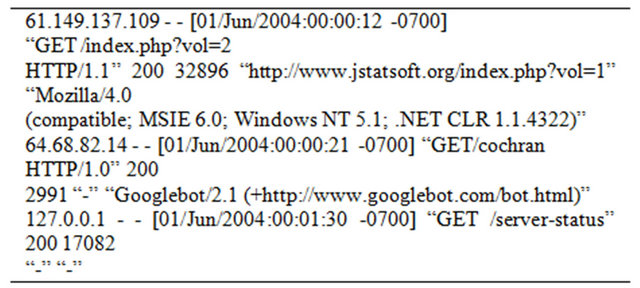
Server log files are the records of transactions, in ASCII format, between the users and the web servers when users access the website. Each line contains the IP address of the remote host making the request for the server, which constitutes the identity of the user, the time of the request, the method of the request, the page requested, the protocol used, the status code, the size of the transactions, the referrer log and the client software making the transaction. Our raw data is the server log file of an academic website, www.stat.ucla.edu, for the whole month of June 2004. The first three lines of our raw data are:
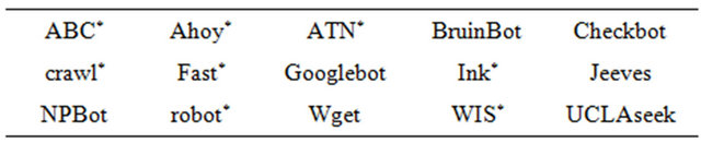
In order to obtain a clean data set with the variable length, we perform several steps. First, we need to remove the action of the robots (machine generated search engines that catalog the Internet) [13]. This will leave out requests of other types, such as figures, plots or files accessible through html documents. Table 1 contains a list of the robots were moved.
After that step, there are only 19,916 lines left
Table 1. List of BOT removed from the raw log file.
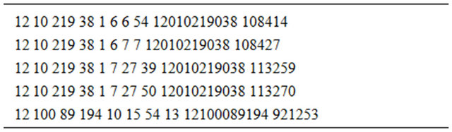
which are the core data we are going to analyze. We then remove most of the information except the IP address and the time in terms of date, hour, minute and second. Now the resultant file is supposed to have 8 columns. The first 4 columns are the IP address, the 5th column is the date and the rest are time (hour/minute/second). The first 5 rows of the data look like the following:

In order to easily compare the IP address and the time, we create two extra columns for numeric IP and generalized time. The numeric IP is to combine the first 4 columns into a 12-number length column, and the generalized time is to combine the last 4 columns into the unit of second since June 1, 00:00:00. This action can be done through either Microsoft Excel or R. The resultant file has its first 5 rows of the data as follow:
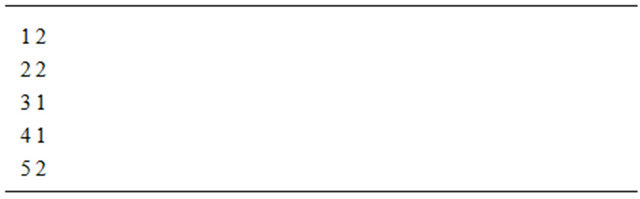
When the generalized columns are done and sorted, we may obtain the length data by analyzing the last 2 generalized columns through. We define the length of one user as the number of page requests of the user from one IP address. We define the so called “same user” under two criteria: First, the IP address is the same. Second, the time between two page requests must be within 20 minutes (1200 seconds). Then the basic idea of this algorithm is as follow. We create a two-column matrix to record the user number (first column) and their corresponding length (second column). The first 5 lines in these data are as follows:
3. A First Look at the Variable Length
A univariate preliminary analysis of length reveals some statistical facts about our UCLA data. The mean number of pages our users visit is 3.043, while the median number of pages is 1. Although among the middle 50% of the users, the number of pages they visit varies only by 2, some rare users visit up to 329 pages within their own sessions.
Figure 1 (left) is the histogram of length for the UCLA data. It possesses several properties that are easily observed. First, sessions tend to be short. Figure 1 (right) magnifies the part of the histogram with lengths from 1 to 10 pages, which cover 95% of all users. Second, the number of users decays exponentially for small values of length. Note that the decay of the number of users is over all lengths, which includes the section of very small lengths shown in Figure 1 (right). In particular, among these 95% of all users who visit less than 10 pages in their sessions, 61% of them visit only 1 page. Third, although the number of users decreases to nearly zero very quickly when length increases, a long tail remains when lengths are larger than 60. In fact, there are 11 rare users (0.17%) who correspond to this long tail. We are not going to consider them as outliers nor try to remove them from the data or any simulations. Exponential behavior at small values of the variable and thick tails suggests power law behavior.
Previous studies suggest that the variable length follows the inverse Gaussian distribution ([7,9]). Theoretically, if a variable x follows the inverse Gaussian distribution, . Taking logarithms on both sides yields
 . In other words, a straight line in a
  versus
  plot with slope close to
  for small values of
![]() , and large values of the variance, is an indication that
, and large values of the variance, is an indication that ![]() follows the inverse Gaussian distribution.
follows the inverse Gaussian distribution.
We can check whether our UCLA data follows inverse Gaussian distribution by the above test. Figure 2 shows the logarithmic number of users versus logarithmic length plot. A linear relationship is shown and can be described by a regression equation:
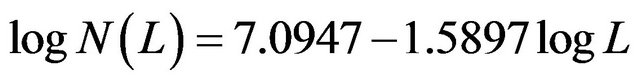 , or equivalently,
 (1)
(1)
where  is the number of users and
 ![]() is length. Note that the slope
is length. Note that the slope  is close to the theoretical value
 . Therefore, this test suggests that the inverse Gaussian distribution is a possible choice for modeling our UCLA data.
4. Comparison Methods for Distributions
This section introduces the several distribution comparison methods we are going to use in the following section.
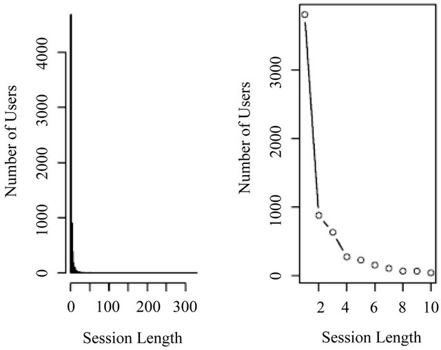
Figure 1. Histogram of UCLA length data. (Left—full histogram; Right—expanded histogram).
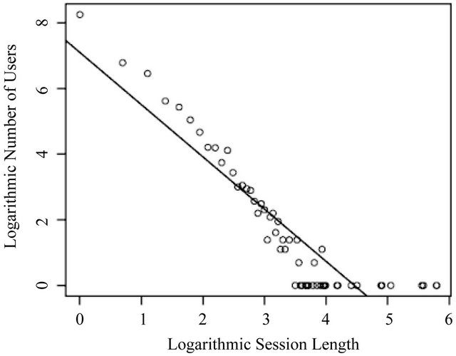
Figure 2. Logarithmic number of users versus logarithmic length plot.
They include: 1) qualitative comparison of the cumulative density functions (CDF) and histograms of the UCLA data and those of simulated session lengths; 2) quantitative comparison of the distributions of the UCLA data and those of simulated session lengths by Kolmogorov-Smirnov test; and 3) quantitative analysis of the long tails of the UCLA data and those of simulated session lengths by skewness and kurtosis.
4.1. Qualitative Comparison of CDF and Histograms
In this qualitative comparison, we compare two sets of session length data: a simulated data set and our UCLA data set. The “simulated data” is generated by a default distribution with parameters obtained via maximum likelihood estimation with the UCLA data. In this paper, we consider the inverse Gaussian and the negative binomial distribution models. We observe the difference of the two data sets’ cumulative density functions and histograms.
The CDF comparison between is done by observing the “simulated-data CDF versus UCLA-data CDF” plot. The “simulated-data CDF” is the cumulative density function of the simulated data and the “UCLA-data CDF” is the cumulative density function of our UCLA data. Ideally, if two CDFs are exactly the same, data points (“o”) will fall onto a solid line with slope 1 and intercept 0. The closer the data points are to the solid line, the more similar are the two CDFs.
The histogram comparison between two different lengths focuses on three main observations: 1) Comparability of the small-length frequencies; 2) Decay behavior in the two histograms; and 3) Comparability of the tails.
4.2. Distribution Comparison by Kolmogorov-Smirnov Test
The two-sample Kolmogorov-Smirnov (KS) test [14], which is a form of minimum distance estimation, is one of the most useful and general nonparametric methods for comparing two data sets, as it is sensitive to differences in both location and shape of the empirical cumulative distribution functions of the two data sets. In this paper, the two-sample KS test serves as a goodness of fit test to compare the simulated data to the UCLA data.
The KS statistic quantifies a distance between the empirical distribution functions of two samples. It is defined as
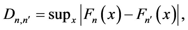 (2)
(2)
where, in our case,  and
and  are the CDF of the simulated data and the UCLA data respectively. Ideally, if two data are exactly the same, we have
 . The null distribution of this statistic is calculated under the null hypothesis that the samples are drawn from the same distribution. The null hypothesis is rejected at level
 .
.
4.3. Long Tail Comparison by Skewness and Kurtosis
Skewness is a measure of symmetry, or more precisely, the lack of symmetry. A distribution with zero skewness is symmetric and it looks the same to the left and right of the center point. Kurtosis is a measure of whether the data are peaked or at relative to a normal distribution. A distribution with high kurtosis tends to have a distinct peak near the mean, decline rather rapidly, and has heavy tails. A distribution with low kurtosis has a flat top near the mean rather than a sharp peak.
Our UCLA data has skewness 23.69 and kurtosis 736.24. Both statistics imply the existence of a long tail. In the following section, we compute the skewness and kurtosis of the simulated data and see how they differ from those of our UCLA data.
5. Data Analysis
The first look at the UCLA data in Section 3 suggests that length follows the inverse Gaussian distribution. In this section, we simulate two sets of length data, one from the inverse Gaussian distribution and another from the negative Binomial distribution, and compare them to our UCLA data. Our objective is to see if conventional models used to fit length work well for the UCLA data.
5.1. The Inverse Gaussian Distribution
The inverse Gaussian (IG) distribution [9] has the probability density function
 (3)
(3)
We simulate an IG data set with the parameters  and
and  obtained from the maximum likelihood estimation applied to the fit of this model to the UCLA data.
Figure 3 shows the simulated-data CDF versus UCLAdata CDF plot. It suggests that there is a small deviation between the two CDFs at the small lengths, but the difference is minimized at the large lengths. In general, the simulated-data CDF underestimates the UCLA-data CDF. The slope and intercept of the regression equation shows the deviation between the two CDFs.
 (4)
(4)
where  and
and  are the CDF of the UCLA data and the simulated data from IG distribution.
Figure 4 shows the comparison of the two histograms. The top histogram is from the UCLA data and the bottom one is from the simulated data, and they are obviously different. First, the height of the first bar is different. Note that most users in the UCLA data set visit only 1 page in their sessions, and the users in the simulated data fail to reproduce this dominance. Second, when length increases, the decay of the number of users in the UCLA data is much faster than that in the simulated data. Third, a long tail does not exist in the simulated data. Based on the histogram of the simulated data, the number of users decays to zero before length reaches 50, which is not the case shown in the histogram of the UCLA data.
A two-sided KS test serves as a goodness-of-fit test on the simulated data. The KS statistic is 0.3549 and the p-value is 0. Therefore, this quantitative test suggests that the simulated data by IG distribution is different from our UCLA data. In addition, the skewness and kurtosis of the simulated data is 2.8839 and 12.4105 respectively. Both of them are much smaller than the statistics of our UCLA

Figure 3. CDF comparison. (“o” as UCLA; “-” as simulated IG data).


Figure 4. Histogram comparison. (Top—UCLA; Bottom— simulated IG data).
data. The skewness suggests that the simulated data is not as skewed as our UCLA data, while the kurtosis suggests that the long tail in the simulated data is not as heavy as the one in our UCLA data. All these quantitative analyses support our observations in the CDF and histogram comparisons.
In summary, our analysis suggests that the data simulated by the IG distribution underestimates the number of users whose lengths are small and fails to simulate those rare users whose lengths are exceptionally large. In addition, when length increases, the decay of the number of users is too slow in the simulated data.
5.2. The Negative Binomial Distribution
The negative binomial (NB) distribution has the probability density function
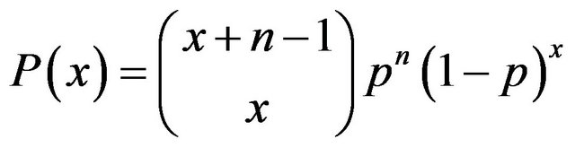 (5)
(5)
where . This distribution is an alternative to the Poisson distribution when the data presents over dispersion, as is the case with the length data. The distribution can also be considered a mixture of a Poisson and a Gamma [15]. We simulate a NB data set with the parameters
  and
and  obtained from the maximum likelihood estimation applied to the UCLA data.
Figure 5 is the simulated-data CDF versus UCLA-data CDF plot. As was the case with the IG distribution, the plot suggests a small deviation between the two CDFs at the small values of length and good fit for large values. In general, the simulated-data CDF still underestimates the UCLA-data CDF. The slope and intercept of the regression equation shows the deviation between the two CDF.
 (6)
(6)
where  is the CDF of the simulated data from NB distribution. However, since the slope is closer to 1 and the intercept is closer to 0, the NB simulated data is closer to our UCLA data than the IG simulated data.
Figure 6 shows the comparison of two histograms. The top histogram represents the UCLA data and the bottom histogram the simulated data; they are still slightly different. First, the height of the first bar in the simulated data histogram is slightly smaller than that in the UCLA data histogram, but this first bar shows a little more dominance in the number of users. Second, although the decay is faster in the simulated data, it still fails to capture the same decay rate as our UCLA data does. Third, a long tail does not exist in the simulated data and the number of users decays to zero before length reaches 50.
The quantitative analysis by the two-sided KS test
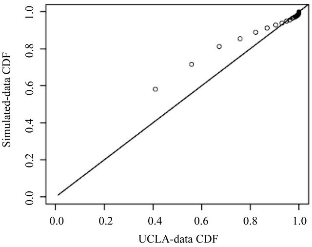
Figure 5. CDF comparison. (“o” as UCLA; “-” as simulated NB data).
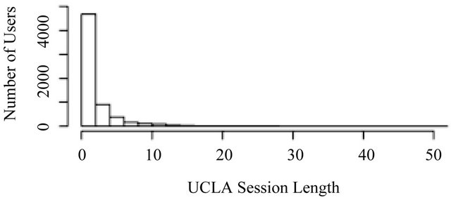
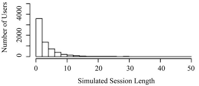
Figure 6. Histogram comparison. (Top—UCLA; Bottom— simulated NB data).
shows that the KS statistic is 0.2293, which is smaller than the KS statistic for the IG simulated data. However, the p-value is still 0, which suggests that the NB distribution is still not good enough to fit our UCLA data. Even worse, the skewness and kurtosis of the simulated data is 1.8200 and 4.6441 respectively. Both of them are much smaller than the statistics of our UCLA data and the IG distribution one. This means that the NB distribution fails to capture the properties of the long tail in our UCLA data.
In summary, our analysis suggests that the NB distribution underestimates the frequency for small values of length, although the underestimation is not as serious as that of the IG distribution. However, rare users whose lengths are fitted better by the NB distribution than that by IG one.
5.3. Discussion
The behavior of users in academic websites is thus no different than that of users in commercial ones. It is universally true that there exists a large group of “incorrectly-entered” users that makes the frequency of the short lengths unusually high. It is also true that there exists a small group of unusual users including robots that creates a long tail in the distribution of length.
Although they share similar characteristics according to the identities of the users, it is not appropriate to conclude the equivalence of them because we do not have data from a commercial website. For example, it is not known whether the decreasing rate of the number of users, out of the total number of users, in the small length is the same in both academic and commercial websites. Further investigation is needed for comparison.
6. A Proposed New Model
The heterogeneity of web browsing data is one of the main features taken into account in most of the literature [4-7]. Recall that www browsing behavior has been modeled, respectively, by whether visitors visit a page or not, by the frequency with which they visit a page, by the sequence of pages visited or by the Markov behavior followed in the visit. It is a common denominator of most research papers using probabilistic models, to consider mixtures models or other forms of cluster analysis to classify visitors [6]. However, no attempts have been made to model the heterogeneity in the length of visits, which, naturally, would be a consequence of the heterogeneous behavior in the other aspects of the visit mentioned above.
Statistical mixture models present two main challenges: first, what is the number of components to use in the mixture (i.e., where to split the whole group); second, what probabilistic model to assume for each component. Researchers in web usage mining usually try different mixtures with different number of components and select the one that best fit the training data [6]. Often, although it is heterogeneity what is being modeled, all the components are assumed to come from the same family, with only different coefficients distinguishing one component from another. This may be a good approach for the other aspects of web browsing considered by researchers, but not for studying length. For the latter, we propose in this section to explore the kind of distribution that best fits the nature of the visitors at each region where length is defined.
The properties of length found in the above sections suggest that we should divide the data into three different groups according to the value of the variable. The first group of data comes from users who either may simply click the wrong website and immediately quit from the website, or know very well what they want in the web site and just look for that. Their behavior explains why lengths in this group of data are unusually small and the frequencies very high but decay exponentially when lengths increase. The number of users who know very well the site is a tiny portion of the overall number of users in this group. The second group of data is the normal (regular) users of our website. Their lengths are small, but not so small when they are compared to the first group of users. Their frequencies decay exponentially. The third group of data comes from users who visit a large number of pages and stay in the website for a long time within one session. It is possible that these users are robots that we fail to eliminate from the data processing, or they are some users who keep clicking our website with strange purposes. Since these users are rare, most frequencies in this group of data are either 0 or 1 and length is unusually large, which results in a very long tail.
6.1. Pareto Distribution
An introduction to Pareto distribution, which appears in the later subsection for modeling, is essential before we continue our discussion on modeling our data. If  is a random variable with a Pareto distribution, then the probability that
  is greater than some number
![]() , i.e. the survival function or tail function, is given by
, i.e. the survival function or tail function, is given by  for
for , or 1 otherwise, where
  is the minimum possible value of
  and
and ![]() is the positive parameter.
is the positive parameter.
Pareto originally used this distribution to describe the allocation of wealth in a society, where a large portion of the wealth of a society is owned by a smaller percentage of people in that society [16]. This idea is commonly called Pareto Principle or the “80-20” rule.
Notice that this distribution is not limited to describing wealth or income, but also to many situations in which an equilibrium is found in the distribution of the “small” to the “large”. The applications include population migration, computer science, physics, astronomy, biology, forest fire, hydrology, etc. [17]. A main common property among these applications is that the variable is related to size, and there exist a lot of small sizes but also a few large sizes. This property exists in our internet traffic data and it is the main reason why we describe our data using Pare to distribution in the following subsections.
6.2. Model Fitting
Inspired by the unique nature of the three groups hypothesized, it is reasonable to divide our data into three groups and fit them separately with three distinct models. Our first group of data features an unusually high frequency at the very small length and a fast exponential decay trend when length increases, so a Pareto distribution is a possible choice for model fitting the low values of length. The probability density function of the Pareto distribution is:
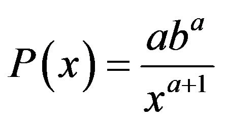 (7)
(7)
where ![]() and
and  are constants. To estimate these parameters, instead of using the traditional maximum likelihood like IG or NB distributions in the previous sections, we suggest to use a data-driven regression analysis on logarithmic number of users and logarithmic length can be used for estimating
 ![]() and
and . In particular, once we have the regression equation in the form of
 , we can obtain
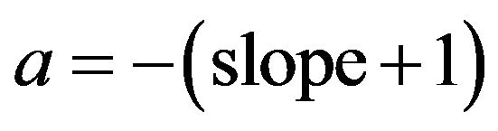 and
and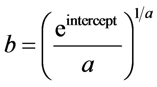 . Therefore, regression analysis suggest that the number of users in the first group can be fitted in terms of lengths by
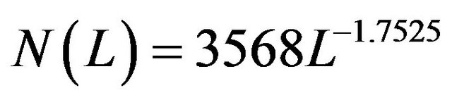 (8)
(8)
for length . The upper limit of this range is chosen so that this group will cover
  of the users.
Our second group of data comes from the normal users of our website. Therefore, it is expected to possess decay properties similar to those of the IG or NB distributions. We suggest fitting also a Pareto distribution. An advantage of using the same distribution is that we can compare the decay rate of the two groups simply by comparing the difference of  of two equations. Regression analysis suggests that the number of users in the second group can be fitted in terms of lengths by
 (9)
(9)
for length . The upper limit of this range is chosen because this is the last nonzero length before at least three consecutive zero number of users.
Our last group of data comes from the long tail feature of length, describing some rare users who visit exceptionally large number of pages within their lengths. Due to its rare existence, it is reasonable to estimate the number of user by
 (10)
(10)
for length , where
 ![]() is a random uniform number between 0 and 1.
is a random uniform number between 0 and 1.  is an indicator function returning 1 if
 , otherwise 0. For our data, the threshold probability is 0.04 because there are 11 rare users having lengths from 55 and 329 in our UCLA data.
6.3. Data Analysis
Once we have fitted our UCLA data with three distinct models, we can combine them into one complete model for simulation. We call this model a “chopped model” because we “chop” the data into three different groups in model fitting. This model can be mathematically presented as
 (11)
(11)
A data it is simulated by this equation in order to compare it to the UCLA data set.
Figure 7 is the simulated-data CDF versus UCLA-data CDF plot. The plot suggests that the difference between the two CDFs is very small for all lengths. A regression equation can be used to describe the relationship of two CDF.
 (12)
(12)
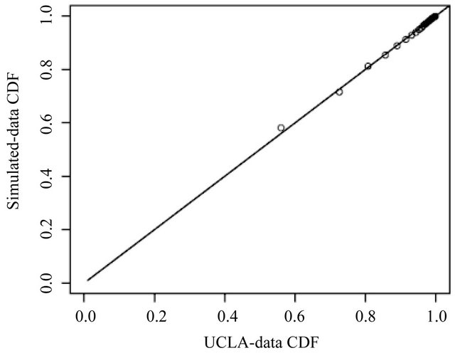
Figure 7. CDF comparison. (“o” as UCLA; “-” as simulated data from chopped model).
where  is the CDF of the simulated data from the chopped model. Note that the slope and the intercept are very close to 1 and 0 respectively, which suggest that the simulated data is very close to our UCLA data.
Figure 8 shows the comparison of two histograms. The top histogram is from UCLA data and the bottom histogram is from the simulated data. They look quite similar according to our three focuses. First, the height of the first bar in the simulated data histogram is very close to that in the UCLA data histogram and it is much higher than the second bar. Second, their decay rates are similar because they both decay near to 0 at around the sixth bar. Third, a long tail exists when length is beyond 50 in both histograms.
The quantitative analysis by two-side KS test shows that the KS statistic is 0.0215, which is the smallest KS statistic we have obtained among three simulated data. The p-value is 0.1022, which suggests that it is difficult to identify the simulated data by our chopped model and our UCLA data by this test with 10% significance level. In addition, the skewness and kurtosis of the simulated data is 35.8689 and 878.5518 respectively. Both of them are very close to the statistics of our UCLA data. This means the simulated data by our chopped model succeeds to capture the long tail property in our UCLA data.
In summary, our analysis suggests that the data simulated by our chopped model succeeds to capture all three properties of our UCLA data, namely exceptionally large number of users in very small lengths, fast decay rate and the existence of long tail in very large lengths.
The performance of our proposed model on an academic website suggests that there may possibly be other, similar models that can fit the data from commercial websites. The key is to identify the nature of the users and divides them into several different groups. Once the groups are divided reasonably well, the combined model may provide a better fit than any other distributions. This

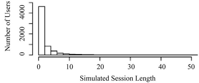
Figure 8. Histogram comparison. (Top—UCLA; Bottom— simulated data from chopped model).
dilemma with the variable length is no different from the dilemma facing those modeling other aspects of web browsing behavior (sequences, choices, ranking, etc.) and the dilemmas faced in using mixture models.
7. Conclusions
We have been concerned in this paper with modeling the behavior of visitors to an academic website. We use raw server log data and focus on the number of links within the site that the visitors browse in one visit. After defining the term “visit” as a session, the units of observation and the variable of interest, we fit to our data the model previously used by the other authors, to reach the same conclusions they obtained with a commercial web site, namely that the data has power law behavior and therefore the modeling could be improved upon by considering other probability models. We try other conventional model but we fail to capture very important features of the data. Finally, we propose a new data-driven modeling approach that fits the data very well.
To measure the goodness of fit of all the models we consistently use qualitative and quantitative measures. The new model is better than the other two considered based on all three measures used. However, the data is chopped in a quite arbitrary manner. More experiments should be performed to search for the optimal chopping positions of the data in order to obtain a better result in model fitting, or otherwise, an automated search algorithm should be implemented for searching these chopping positions. All these works are considered as future researches extended from this work.
Although our new model fits the data well, it is an exploratory model in need of further formalization once more data are available. It would be interesting to see its behavior with other web sites to determine how useful it could be to web managers and e-commerce in general. It would also be interesting to see how, assuming such a behavioral model, changes the analysis of other aspects of web browsing behavior, such as sequences followed in a visit, entry page, and other aspects of web browsing of web browsing that previous authors have considered but did not concern us here.
This is the subject of our future research to apply the model to new data sets. For example, one recent work related to the method mentioned in this paper is [18]. These applications to new models allow us to obtain a more general model where the determination of the optimal length at which to chop would be done simultaneously with the estimation of the parameters of the different pieces of the model.
8. Acknowledgement
The authors thank to the Department of Statistics at UCLA for kindly providing the raw data. This work was supported by National Science Council of Taiwan grant number 100-2118-M-001-002-MY2.
REFERENCES
- J. Srivastava, R. Cooley, D. Mujund and P. N. Tan, “Web Usage Mining: Discovery and Applications of Usage Patterns from Web Data,” SIGKDD Explorations, Vol. 1, No. 2, 2000, pp. 12-23. doi:10.1145/846183.846188
- J. Sanchez and Y. He, “Internet Data Analysis for the Undergraduate Statistics Curriculum,” Journal of Statistics Education, Vol. 13, No. 3, 2005, pp. 1-20.
- M. Eirinaki and M. Vazirgiannis, “Web Mining for Web personalization,” ACM Transactions on Internet Technology, Vol. 3, No. 1, 2003, pp. 1-27. doi:10.1145/643477.643478
- S. Park, N. C. Suresh and B. Jeong, “Sequence-Based Clustering for Web Usage Mining: A New Experimental Framework and ANN-Enhanced K-Means Algorithm,” Data & Knowledge Engineering, Vol. 65, No. 3, 2008, pp. 512-543. doi:10.1016/j.datak.2008.01.002
- J. G. Dias and J. K. Vermunt, “Latent Class Modeling of Website Users’ Search Patterns: Implications for Online Market Segmentation,” Journal of Retailing and Consumer Services, Vol. 14, No. 6, 2007, pp. 359-368. doi:10.1016/j.jretconser.2007.02.007
- P. Baldi, P. Frasconi and P. Smyth, “Modeling the Internet and the Web: Probabilistic Methods and Algorithms,” John Wiley and Sons Ltd., Hoboken, 2003.
- R. Sen and M. Hansen, “Predicting Web Users Next Access Based on Log Data,” Journal of Computational and Graphical Statistics, Vol. 12, No. 1, 2003, pp. 143-155.
- I. Cadez, D. Heckerman, C. Meek, P. Smyth and S. White, “Model-Based Clustering and Visualization of Navigation Patterns on a Web Site,” Journal of Data Mining and Knowledge Discovery, Vol. 7, No. 4, 2003, pp. 399-424. doi:10.1023/A:1024992613384
- B. A. Huberman, P. L. T. Pirolli, J. E. Pitkow and R. M. Lukose, “Strong Regularities in World Wide Web Surfing,” Science, Vol. 280, No. 3, 1998, pp. 95-97. doi:10.1126/science.280.5360.95
- D. Heckerman, “The UCI KDD Archive,” Department of Information and Computer Science, University of California, Oakland, 2013. http://kdd.ics.uci.edu/databases/msnbc/msnbc.data.html
- J. Eason and J. Johannesen, “Meaningful Data from Web Logs,” Proceedings of the Twenty-Ninth Annual SAS Users Group International Conference (SUGI 29), SAS Institute Inc., Cary, 2004.
- J. Callender, “Perl for Web Site Management,” O’Reilly, Sebastopol, 2001.
- “Robots Database,” 2008. http://www.robotstxt.org/db.html
- I. M. Chakravarti, R. G. Laha and J. Roy, “Handbook of Methods of Applied Statistics, Volume I,” John Wiley and Sons, Hoboken, 1967, pp. 392-394.
- J. M. Hilbe, “Negative Binomial Regression,” Cambridge University Press, Cambridge, 2007. doi:10.1017/CBO9780511811852
- V. Pareto, “Cours d’Economie Politique: Nouvelle Edition par G.-H. Bousquet et G. Busino,” Librairie Droz, Geneva, 1964, pp. 299-345.
- W. J. Reed and M. Jorgensen, “The Double Pareto-Lognormal Distribution—A New ParametricModel for Size Distributions,” Communications in Statistics: Theory and Methods, Vol. 33, No. 8, 2004, pp. 1733-1753. doi:10.1081/STA-120037438
- F. K. H. Phoa and W. C. Liu, “High-Quality Winners Take More: Modeling Non-Scale-Free Bulletin Forums with Content Variations,” Journal of Data Science, in Press, 2013.