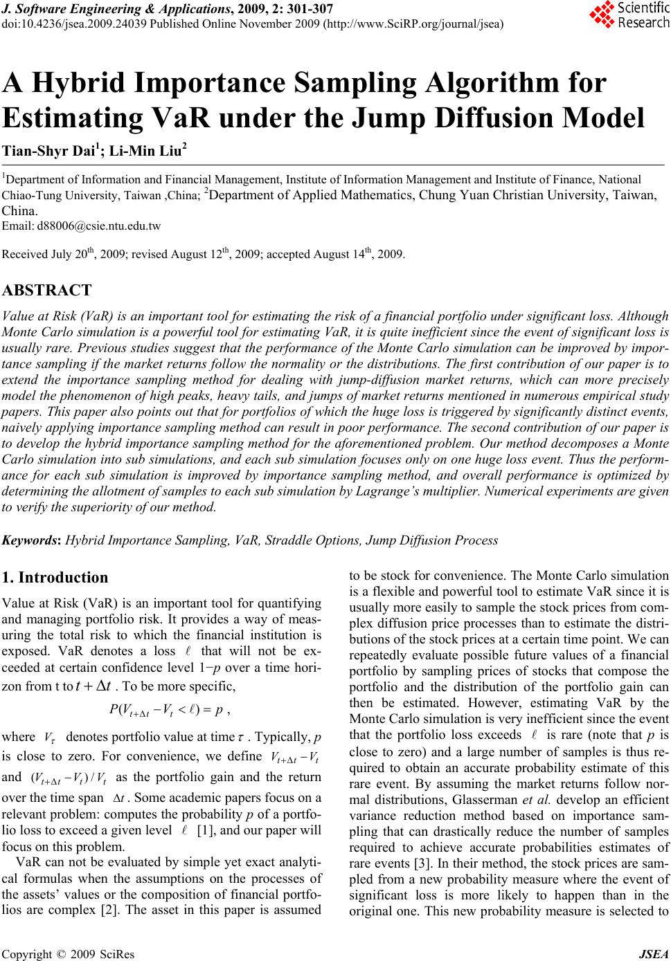J. Software Engineering & Applications, 2009, 2: 301-307
doi:10.4236/jsea.2009.24039 Published Online November 2009 (http://www.SciRP.org/journal/jsea)
301
A Hybrid Importance Sampling Algorithm for
Estimating VaR under the Jump Diffusion Model
Tian-Shyr Dai1; Li-Min Liu2
1Department of Information and Financial Management, Institute of Information Management and Institute of Finance, National
Chiao-Tung University, Taiwan ,China; 2Department of Applied Mathematics, Chung Yuan Christian University, Taiwan,
China.
Received July 20th, 2009; revised August 12th, 2009; accepted August 14th, 2009.
ABSTRACT
Value at Risk (VaR) is an important tool for estimating the risk of a financial portfolio under significant loss. Although
Monte Carlo simulation is a powerful tool for estimating VaR, it is quite inefficient since the event of significant loss is
usually rare. Previous studies suggest that the performance of the Monte Carlo simulation can be improved by impor-
tance sampling if the market returns follow the normality or the distributions. The first contribution of our paper is to
extend the importance sampling method for dealing with jump-diffusion market returns, which can more precisely
model the phenomenon of high peaks, heavy tails, and jumps of market returns mentioned in numerous empirical study
papers. This paper also points out that for portfolios of which the huge loss is triggered by significantly distinct events,
naively applying importance sampling method can result in poor performance. The second contribution of our paper is
to develop the hybrid importance sampling method for the aforementioned problem. Our method decomposes a Monte
Carlo simulation into sub simulations, and each sub simulation focuses only on one huge loss event. Thus the perform-
ance for each sub simulation is improved by importance sampling method, and overall performance is optimized by
determining the allotment of samples to each sub simulation by Lagrange’s multiplier. Numerical experiments are given
to verify the superiority of our method.
Keywords: Hybrid Importance Sampling, VaR, Straddle Options, Jump Diffusion Process
1. Introduction
Value at Risk (VaR) is an important tool for quantifying
and managing portfolio risk. It provides a way of meas-
uring the total risk to which the financial institution is
exposed. VaR denotes a loss that will not be ex-
ceeded at certain confidence level 1−p over a time hori-
zon from t to. To be more specific,

tt
()
tt t
PV Vp
 ,
where V

denotes portfolio value at time

. Typically, p
is close to zero. For convenience, we define tt t VV


and as the portfolio gain and the return
over the time span Some academic papers focus on a
relevant problem: computes the probability p of a portfo-
lio loss to exceed a given level  [], and our paper will
focus on this problem.
(
tt ) t t
VV/V
1
t.
VaR can not be evaluated by simple yet exact analyti-
cal formulas when the assumptions on the processes of
the assets’ values or the composition of financial portfo-
lios are complex [2]. The asset in this paper is assumed
to be stock for convenience. The Monte Carlo simulation
is a flexible and powerful tool to estimate VaR since it is
usually more easily to sample the stock prices from com-
plex diffusion price processes than to estimate the distri-
butions of the stock prices at a certain time point. We can
repeatedly evaluate possible future values of a financial
portfolio by sampling prices of stocks that compose the
portfolio and the distribution of the portfolio gain can
then be estimated. However, estimating VaR by the
Monte Carlo simulation is very inefficient since the event
that the portfolio loss exceeds is rare (note that p is
close to zero) and a large number of samples is thus re-
quired to obtain an accurate probability estimate of this
rare event. By assuming the market returns follow nor-
mal distributions, Glasserman et al. develop an efficient
variance reduction method based on importance sam-
pling that can drastically reduce the number of samples
required to achieve accurate probabilities estimates of
rare events [3]. In their method, the stock prices are sam-
pled from a new probability measure where the event of
significant loss is more likely to happen than in the
original one. This new probability measure is selected to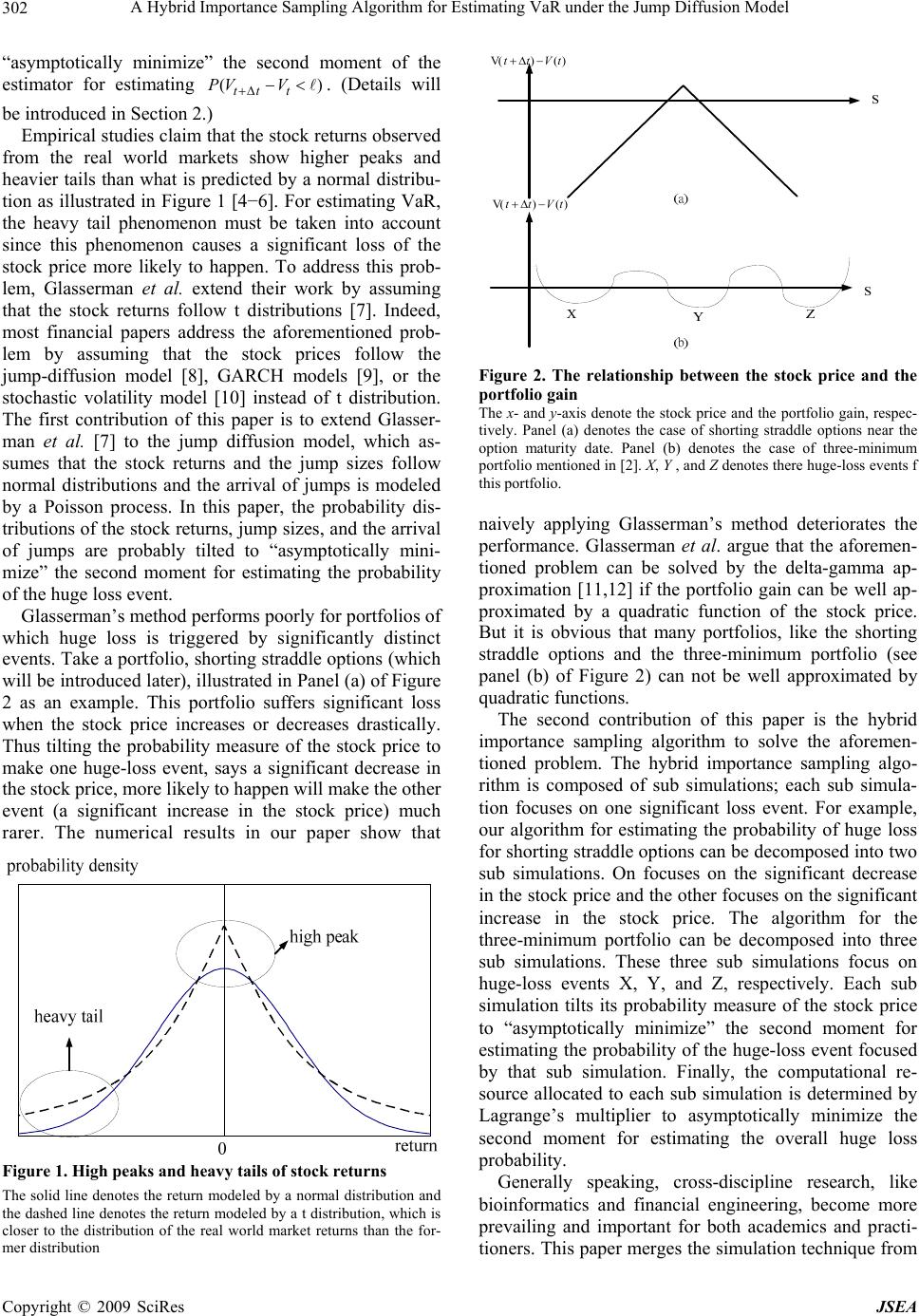


A Hybrid Importance Sampling Algorithm for Estimating VaR under the Jump Diffusion Model 302
“asymptotically minimize” the second moment of the
estimator for estimating . (Details will
be introduced in Section 2.)
(
tt t
PV V
 )
Empirical studies claim that the stock returns observed
from the real world markets show higher peaks and
heavier tails than what is predicted by a normal distribu-
tion as illustrated in Figure 1 [4−6]. For estimating VaR,
the heavy tail phenomenon must be taken into account
since this phenomenon causes a significant loss of the
stock price more likely to happen. To address this prob-
lem, Glasserman et al. extend their work by assuming
that the stock returns follow t distributions [7]. Indeed,
most financial papers address the aforementioned prob-
lem by assuming that the stock prices follow the
jump-diffusion model [8], GARCH models [9], or the
stochastic volatility model [10] instead of t distribution.
The first contribution of this paper is to extend Glasser-
man et al. [7] to the jump diffusion model, which as-
sumes that the stock returns and the jump sizes follow
normal distributions and the arrival of jumps is modeled
by a Poisson process. In this paper, the probability dis-
tributions of the stock returns, jump sizes, and the arrival
of jumps are probably tilted to “asymptotically mini-
mize” the second moment for estimating the probability
of the huge loss event.
Glasserman’s method performs poorly for portfolios of
which huge loss is triggered by significantly distinct
events. Take a portfolio, shorting straddle options (which
will be introduced later), illustrated in Panel (a) of Figure
2 as an example. This portfolio suffers significant loss
when the stock price increases or decreases drastically.
Thus tilting the probability measure of the stock price to
make one huge-loss event, says a significant decrease in
the stock price, more likely to happen will make the other
event (a significant increase in the stock price) much
rarer. The numerical results in our paper show that
Figure 1. High peaks and heavy tails of stock returns
The solid line denotes the return modeled by a normal distribution and
the dashed line denotes the return modeled by a t distribution, which is
closer to the distribution of the real world market returns than the for-
mer distribution
)()V( tVtt



)()V( tVtt



Figure 2. The relationship between the stock price and the
portfolio gain
The x- and y-axis denote the stock price and the portfolio gain, respec-
tively. Panel (a) denotes the case of shorting straddle options near the
option maturity date. Panel (b) denotes the case of three-minimum
portfolio mentioned in [2]. X, Y , and Z denotes there huge-loss events f
this portfolio.
naively applying Glasserman’s method deteriorates the
performance. Glasserman et al. argue that the aforemen-
tioned problem can be solved by the delta-gamma ap-
proximation [11,12] if the portfolio gain can be well ap-
proximated by a quadratic function of the stock price.
But it is obvious that many portfolios, like the shorting
straddle options and the three-minimum portfolio (see
panel (b) of Figure 2) can not be well approximated by
quadratic functions.
The second contribution of this paper is the hybrid
importance sampling algorithm to solve the aforemen-
tioned problem. The hybrid importance sampling algo-
rithm is composed of sub simulations; each sub simula-
tion focuses on one significant loss event. For example,
our algorithm for estimating the probability of huge loss
for shorting straddle options can be decomposed into two
sub simulations. On focuses on the significant decrease
in the stock price and the other focuses on the significant
increase in the stock price. The algorithm for the
three-minimum portfolio can be decomposed into three
sub simulations. These three sub simulations focus on
huge-loss events X, Y, and Z, respectively. Each sub
simulation tilts its probability measure of the stock price
to “asymptotically minimize” the second moment for
estimating the probability of the huge-loss event focused
by that sub simulation. Finally, the computational re-
source allocated to each sub simulation is determined by
Lagrange’s multiplier to asymptotically minimize the
second moment for estimating the overall huge loss
probability.
Generally speaking, cross-discipline research, like
bioinformatics and financial engineering, become more
prevailing and important for both academics and practi-
tioners. This paper merges the simulation technique from

A Hybrid Importance Sampling Algorithm for Estimating VaR under the Jump Diffusion Model 303
applied mathematics and algorithm design and perform-
ance comparisons knowhow from computer science dis-
cipline to develop efficient numerical programs to solve
finance problem. It plays a great platform to interchange
the ideas, the challenges, and the techniques among the
computer scientists, mathematicians, and financial ex-
perts.
The paper is organized as follows. The assumptions of
the Merton’s jump diffusion model, the Glasserman’s
importance sampling method, and the definitions of
straddle options are introduced in Section 2. In Section 3,
we will use shorting straddle options as an example to
demonstrate how the probabilities of the jump diffusion
process are tilted for each sub simulation and how the
number of samples is allocated to each sub simulation to
optimize the overall performance. Numerical results in
Section 4 verify the superiority of our method. Section 5
concludes the paper.
2. Preliminaries
2.1 The Stock Price Process
Define St as the stock price at year t. Under the Merton’s
jump diffusion model, the stock price process can be
expressed as
(1)
X
t
t
t
dS dtdW edN
S


 t (1)
where is the standard Wiener process, μ is the aver-
age stock return per annum, σ is the annual volatility, X is
a normal random variable that models the jump size, and
t
W
t
N
denotes the Poisson process. We further assume
that 2 ,)~(XN

 and (1)
t
PdN dt


t
. Define the stock
return over the time horizonas follows:
1
,
t
N
tt t
t
ti
SS
rttZ
S






i
Z
(2)
where


~0,1ZN , t
N


denotes the number of jumps be-
tween time t and , tt 2 ~(,)
i
ZN

 . Note that the
aforementioned model degenerates into the Black- Scho-
les lognormal diffusion process [13] when λ = 0 (i.e.
in Equation (2)).
0
t
N
2.2 Glasserman’s Importance Sampling Method
This subsection sketches Glasserman’s importance sam-
pling method [3] by assuming that the stock price process
follows the log-normal diffusion process. Consider a
portfolio which is composed of a stock. Let A denotes the
event that the portfolio gain is less than:



()() 0
S()-S()
=0
() ()
=0 (3)
()
=-0 (
t
tp
ASt tSt
ttt
St St
rSt
rr

  











4)
=Z: f(Z)-0 (5)
tp p
rrttZr   
where we substitute Equation (2) into Equation (3) and
(5), andp
t
rS

into Equation (4).
To minimize the second moment for estimating the
probability of event A, Glasserman samples Z from a new
probability measure


instead of the original prob-
ability measure

(where


~0,1ZN ). The likelihood
ratio for these two probabilities measures is

exp()() ,
dfZ
d





 (6)
where Ψ(θ) ≡ logE [exp (θf(Z))]. Define E


as the
expected value measured under

 and


:( )0,
p
AZfZttZr
 
 
where ~(,1)
Z
Nt

 . Then we have
*9(1 )1exp(()()) .
AA dpE EfZ




 

The second moment of the estimator is then
Second moment
1exp( 2()2( ))exp(2()).
A
EfZ







 (7)
To asymptotically optimize the performance of the
Monte Carlo simulation, a proper θ is selected to mini-
mize exp (2Ψ(θ)) by the following equation:
'() 0


 (8)


is then determined by substituting θ (obtained
from Equation (8)) into Equation (6).
2.3 Straddle Options
Stock options are derivative securities that give their
buyer the right, but not the obligation, to buy or sell the
underlying stocks for a contractual price called the exer-
cise price K at maturity. Assume that the options mature
at timett

 then the payoffs of a call option and a put
option at maturity are maxand max

,0
tt
SK
 



KS,0
tt, respectively. Shorting straddle options
denotes a portfolio that shortsunits call options and
1
D

A Hybrid Importance Sampling Algorithm for Estimating VaR under the Jump Diffusion Model 304
2
D units put options with the same strike price. To be
more specific, the portfolio gain at maturity is




12
max,0 max,0
tt tt
DSKD KS
 
. The portfo-
lio gain is interpreted in terms of stock returndefined
Equation (2) in Figure 3. Note that
t
r
*
0t
t
K
S
rS

 (9)
The portfolio gain can be expressed as follows:
Portfolio Gain(10)
**
02010
*
2t
(),
, ,
tt t
tt
rSrrSifr
rSifr







*
0
,
1
t
r
r


where 1
D

 and 2 D2


t
r
. The portfolio gain is less
than if the stock returnis larger thanor lower than
, where
*
1
r
*
2
r
**
*0201
1
1
tt
t
rS rS
rS




and *
2
2
.
t
rS


t
3. Contributions
We will use shorting straddle options as an example to
illustrate the major contributions of this paper. First, the
huge loss events of this portfolio are identified. The
Monte Carlo simulation is then decomposed into two sub
simulations; each focuses on one huge loss event. Next,
the probability distribution for each sub simulation is
tilted to asymptotically minimize the second moment of
the estimator under the jump diffusion assumption. Fi-
nally, the allotment of samples for each sub simulation is
determined by Lagrange’s multiplier to optimize the
overall performance.
3.1 Identify the Huge Loss Events
In Figure 3, the portfolio gain of shorting straddle op-
tions is less than when the stock return exceeds
threshold or is below
r
*
1
r
*
2
r. For convenience, events1
A
and 2
A
are used to denote the events


*
1t
rr and


*
2
r
t
r,
respectively, as follows:


**
1102 01
:()( )
tt t
Arfr rrrr  
*
0,
,
(11)

*
22 2
:()0
ttt
Arfrr r  
where and formula
*/t
rS1()
t
f
rand 2()
t
f
rare derived
from Equation (10). Since1
A
and 2
A
are mutually exclusive,
the probability that the portfolio gain is less than is 
1


121 2
11
AAAA
pEE E




.
The Monte Carlo simulation for estimating p can be
decomposed into two sub simulations; one focuses on
event 1
A
, and the other one focuses on event2
A
.
3.2 Importance Sampling under the Jump
Diffusion Assumption
Next, we will describe how to efficiently estimate1 1
A
E




and 2 1A E



by importance sampling. Assume that the sub
simulations for estimatingand tilt their
probabilities from
1
1A E
 2
1A E


to 1

 and2

, respectively.
Then 1

and 2

are derived as follows: Define
11
() log 11 (
t
e ))Efrxp( 




))
t
fr
and .
22
(22 ( ))
t
fr 

) logexp(E  
11
exp( (E 



 can be calculated as follows:
**
1110210 1
***
102101111
exp(())exp(())
= exp(-)(exp()).
tt
t
EfrE rrrr
rrrE r

 
*







 
Note that
11 11
1
(exp())exp( ())
t
N
ti
i
ErE ttZZ  






 





222
111 111
1
exp(0.5)exp()'
Nt
i
i
ttE Z  



  



11 11
10 1
222
1111
0
222
111 1
0
exp( )exp( )
!
=exp(0.5
!
( exp(0.5))
=!
t t
t
t
Nnn
t
ii
in i
n
t
n
n
t
n
e
EZ EZ
n
enn
n
e
n




 


 

 
 









 







 


222
1111
0.5
t
=exp(),
t
e
  

 
where tt



. Thus 1

can be obtained by numerically
solving the equation '
11
() 0 

 (see Equation (8)) as
follows:
'*** 22
1102 01111
22 222
11111 11
()
()exp(0.5)0.
t
rrrt t 
 




Similarly, it can be derived that
222
2222
22
22222 2
0.5 *
2
exp(())exp(0.5
).
t
tt
Efrt t
re
  
2




 

 



2

can also be solved numerically by the equation
'
22
 ()0

as follows:

A Hybrid Importance Sampling Algorithm for Estimating VaR under the Jump Diffusion Model 305
)()V( tVtt 

t
r
2
slope
t
S


1
slope
t
S


*
0
r
*
2
r
*
1
r
Figure 3. Shorting straddle options
The x- and y-axis denote the stock return and the portfolio gain, respectively.
222
2222
'22
22 222
0.5 22
22 2
()
()
t
tt r
e
  




 
*
0.
Finally, the new probability distribution1

sampled
by the first sub simulation can be derived by Equation (6)
as follows:





1
2
1
22
222
0.5
211 222
11
111 1
11
111 1
()
/2 2111 1
2
0
0.5
2
2
exp(( )())
11
= exp
!
22
11
=
!
22
n
kK
t
t
t
nZ
n
Zt
t
n
n
e
Zt t
dd fr
e
eefr
n
ee
en
  




  

















 

















2
2
111
2
2
0
.
n
kK
Z
n
n
e





 
 
 

 
 
 


That is, the first sub simulation tilts the probability
from to
1

, where the distributions of random vari-
ables defined in Equation (2) are changed as follows:


11
~,1
Z
Nt  


222
111 1
0.5
~
tt
NPoissone
 


 and


22
11
~
i
ZN
 


11111 11
11exp
At
EEA fr









.
Thus 1
1A E



 is estimated by sampling the unbiased es-
timator

 


111 1
xp
At
fr
1
1e

 
from1

in the first
,

  .
Note that
sub simulation. Similarly, the probability distribution
2


used by the second sub simulation can be derived as







2
222 2
0.5
222 2
222 22 122
2222
22
2
222 2
0.5
2 2
2
0
exp
11
=.
!
22
n
tKK
t
eZ
n
Zt t
n
dd fr
ee
ee
n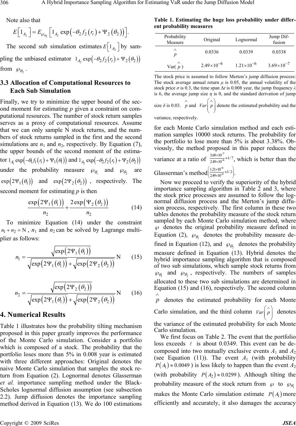



 













 













A Hybrid Importance Sampling Algorithm for Estimating VaR under the Jump Diffusion Model 306
Note also that



22
2222 2
11exp
AA t
EE fr





 
.
The second sub simulation estimatesby sam-
pling the unbiased estimator
2
1A E

  

22 2
1exp
At
 
22
fr
from 2

.
3.3 Allocation of Computational Resources to
Each Sub Simulation
Finally, we try to minimize the upper bound of the sec-
ond moment for estimating p given a constraint on com-
putational resources. The number of stock return samples
serves as a proxy of computational resources. Assume
that we can only sample N stock returns, and the num-
bers of stock returns sampled in the first and the second
simulations are n1 and n2, respectively. By Equation (7),
the upper bounds of the second moment of the estima-
tor
 

1111 1
1exp
At
fr

  and
 


2222 2
1exp
At
fr  
1

under the probability measure

2 and


are




11
p 2ex

 and




22
 exp 2, respectively. The
second moment for estimating p is then
   
112 2
22
exp22 exp
nn
 
 (14)
To minimize Equation (14) under the constraint
, n1 and n2 can be solved by Lagrange multi-
plier as follows:
12
Nnn






11
1
112 2
exp 2
N
exp 2exp2
n



 (15)
 




22
2
11
exp 2
2 2
N
exp 2exp2
n
 


 (16)
4. Numerical Results
Table 1 illustrates how the probability tilting mechanism
proposed in this paper greatly improves the performance
of the Monte Carlo simulation. Consider a portfolio
which is composed of a stock. The probability that the
portfolio loses more than 5% in 0.008 year is estimated
with three different approaches: Original denotes the
naive Monte Carlo simulation that samples the stock re-
turn from Equation (2). Lognormal denotes Glasserman
et al. importance sampling method under the Black-
Scholes lognormal diffusion assumption (see subsection
2.2). Jump diffusion denotes the importance sampling
method derived in Equation (13). We do 100 estimations
Table 1. Estimating the huge loss probability under differ-
ent probability measures
Probability
Measure Original Lognormal
Jump Dif-
fusion
p

0.0336 0.0339 0.0338
Var(
p

) 6
2.49 10

 6 1.21 10  7 3.69 10


The stock price is assumed to follow Merton’s jump diffusion process:
The stock average annual return μ is 0.05, the annual volatility of the
stock price σ is 0.3, the time span Δt is 0.008 year, the jump frequency λ
is 6, the average jump size η is 0, and the standard derivation of jump
size δ is 0.03.
p

and Varp





denote the estimated probability and the
variance, respectively.
for each Monte Carlo simulation method and each esti-
mation samples 10000 stock returns. The probability for
the portfolio to lose more than 5% is about 3.38%. Ob-
viously, the method proposed in this paper reduces the
variance at a ratio of
7
6
3.69 101/7
2.49 10



, which is better than the
Glasserman’s method
6
6
1.21 101/ 2
2.49 10








.
Now we proceed to verify the superiority of the hybrid
importance sampling algorithm in Table 2 and 3, where
the stock price processes are assumed to follow the log-
normal diffusion process and the Merton’s jump diffu-
sion process, respectively. The first column in these two
tables denotes the probability measure of the stock return
sampled by each Monte Carlo simulation method, where

denotes the original probability measure defined in
Equation (2), 1


denotes the probability measure de-
fined in Equation (12), and 2

 denotes the probability
measure defined in Equation (13). Hybrid denotes the
hybrid importance sampling algorithm that is composed
of two sub simulations, which sample stock returns from
1


and 2


, respectively. The numbers of samples
allocated to these two sub simulations are determined in
Equation (15) and (16), respectively. The second column
p

denotes the estimated probability for each Monte
Carlo simulation, and the third column Var p





denotes
the variance of the estimated probability for each Monte
Carlo simulation.
We first focus on Table 2. The event that the portfolio
loss exceeds is about 0.0349. This event can be de-
composed into two mutually exclusive events A1 and A2
(see Equation (11)). The event A
1 (with probability



10.0049PA ) is less likely to happen than the event A2
(with probability


20.0299PA ). Although tilting the
probability measure of the stock return from

to 1


makes the Monte Carlo simulation estimate


1
PA more
efficiently and accurately, it also damages the accuracy

A Hybrid Importance Sampling Algorithm for Estimating VaR under the Jump Diffusion Model 307
for estimating. It can be observed that this tilting
produce inaccurate probability estimation (0.0139) with
large variance. Similar problem applies to the Monte
Carlo simulation that tilts the probability measure to

2
PA
2

; this Monte Carlo simulation is inadequate to esti-
mate . But tilting the probability measure to

1
PA 2


is better than tilting the probability to1

since the event
A2 constitutes the bulk of the event that the portfolio loss
exceeds . Note that both important sampling methods
mentioned above are less efficient than the primitive
Monte Carlo simulation (that samples the stock return
form ). On the other hand, the hybrid importance
sampling algorithm performs better than the primitive
Monte Carlo simulation. It produces accurate probability
estimation and reduces the variance at a ratio of


7
6
2.28 10
3.55 10







1/1
5


stock return to 1 P

(or 2 P

) also performs poorly in this
case. Note that the hybrid importance sampling algorithm
still outperforms the primitive Monte Carlo simulation by
reducing the variance at a ratio of
7
6
5.44 10
1/7.5
4.05 10




 



.
5 Conclusions
The paper improves the performance for estimating VaR.
We first extend Glasserman’s importance sampling
method to Merton’s jump diffusion process. Then we
suggest a novel Monte Carlo simulation, the hybrid im-
portance sampling algorithm, which can efficiently esti-
mate the VaR of complex financial portfolios. Numerical
results given in this paper verify that our method greatly
improve the performance.
6. Acknowledgement


. In other words, the sample size of the
primitive Monte Carlo simulation should be 15 times the
sample size of the hybrid importance sampling algorithm
to make the former method achieve the same accuracy
level as the latter method.
We thank Shi-Gra Lin, and Ren-Her Wang for useful
suggestions.
REFERENCES
[1] S. K. Lin, C. D. Fuh, and T. J. Ko, “A bootstrap method
with importance resampling to evaluate value-at-risk,” J.
Financial Studies, Vol. 12, pp. 81–116, 2004.
In Table 3, the probability that the portfolio loss ex-
ceeds is larger (about 0.0403) since the jumps in stock
price make the huge loss events A1 and A2 more likely to
happen. Naively tilting the probability measure of the [2] H. G. Fong and K. C. Lin, “A new analytical approach to
value at risk,” J. Portfolio Management, Vol. 25, pp.
88–97, 1999.
Table 2. Compare monte carlo simulations under the log-
normal stock price model [3] P. Glasserman, P. Heidelberger, and P. Shahabuddin,
Vaniance Reduction Technique for Estimating Value-at-
Risk, Management Sci., Vol. 46, pp. 1349–1364, 2000.
Prob-
ability
Meas-
ure
1

 Hybrid
2


p

[4] E. Eberlein, U. Keller, and K. Prause, “New insights into
smile, mispricing, and value-at-risk: The hyperbolic
model, J. Business, Vol. 71, pp. 371–406, 1998.
0.0349 0.0139 0.0395 0.0349
[5] J. R. M. Hosking, G. Bonti, and D. Siegel, “Beyond the
Lognormal,” Risk, Vol. 13, pp. 59–62, 2000.
p
36
55 10 . 3 4.14 10

 3 2.5 7 2 10 2.28 10


Var( )
[6] K. Koedijk, R. Huisman, and R. Pownall, “VaR-x: Fat tails
in financial risk management,” J. Risk 1, pp. 47–62, 1998.
Consider a short straddle option that contains a short position in 1 unit
call option

and 1 unit put option

. The probability
for the portfolio to lose more than 5% of the stock price in 0.008 year is
estimated in column 2 (i.e.,and ). The stock av-
erage annual return μ is 0.05, the annual volatility of the stock price σ is
0.3, anddefined in Equation (9) is 0.01. Note that the jump fre-
quency λ is 0 in this case.
 
11
  21
0.05S

t

*0.05r
[7] P. Glasserman, P. Heidelberger, and P. Shahabuddin,
“Portfolio value-at-risk with heavy-tailed risk factors,”
Math. Finance, Vol. 12, pp. 239–269, 2002.
[8] R. C. Merton, “Option pricing when underlying stock
returns are discontinuous,” J. Financial Econ., Vol. 3, pp.
125–144, 1976.
*
0
r
[9] J.-C. Duan, “The GARCH option pricing model,” Math.
Finance, Vol. 5, pp. 13–32, 1995.
Table 3. Compare monte carlo simulations under the mer-
ton’s jump diffusion stock price model
[10] S. Heston, “A closed-form folution for options with stochas-
tic volatility with applications to bond and currency op-
tions,” Rev. Financial Studies, Vol. 6, pp. 327–343, 1993.
Prob-
ability
Meas-
ure
 1

 2

 Hybrid
p

0.0405 0.0363 0.0426 0.0403
Var(
[11] P. Jorion, Value at risk, McGraw-Hill, New York, 1997.
[12] C. Rouvnez, Going Greek with VaR, Risk 10 (1997)
57–65.
p

) 6
4.05 10  2 1.97 10
s

 4 6.2 7 1 10 5.44 10

[13] F. Black and M. Scholes, “The pricing of options and
corporate liabilities,” J. Political Econ., Vol. 81, pp.
637–659, 1973.
The numerical settings follow the settings listed in Table 2 except that
the jump frequency λ is 6, the mean of jump size η is 0, and the stan-
dard derivation of jump size δ is 0.03.