American Journal of Oper ations Research, 2011, 1, 284-292
doi:10.4236/ajor.2011.14033 Published Online December 2011 (http://www.SciRP.org/journal/ajor)
DEA Models for the Efficiency Evaluation of System
Composed of Parallel Subsystems
Jinnian Wang*, Yongjun Li
School of Management, University of Science and Technology of China, Hefei, China
Received August 30, 2011; revised Septembe r 27, 2011; acc ept ed Oct ober 9, 2011
Abstract
The perspective of internal structure of the decision making units (DMUs) was considered as the “black box”
when employing data envelopment analysis (DEA) models. However, in the actual world there are always
some DMUs that are composed of several sub-units or subsystems, each utilizes the same inputs to generate
same outputs. Numerous instances can be listed, such as a firm with a few of plants. In this paper we present
models that evaluated the efficiency of DMU which is comprised of same several parallel subsystems, the
foremost contribution of our work is that we take the different importance of the subsystems into account in
the model, which can be obviously distinguished to the existing DEA model. Secondly, since the alternative
optimal multipliers may emerge in the model, the efficiency of each subsystem may be non-unique and we
simultaneously develop models of efficiency decomposition for each subsystem. At last a case of technologi-
cal innovation activities of each province in China is used as an example to state the models.
Keywords: Data Envelopment Analysis, Parallel Subsystems, Efficiency Decomposition, Technological
Innovation
1. Introduction
A non-parametric mathematical programming, data en-
velopment analysis (DEA), has been widely used in per-
formance evaluation and benchmark [1]. Since the ap-
pearance of first CCR model [2], a series of different
DEA models, such as BCC [3], FG [4], ST [5] and so on,
have been proposed in succession. The method has been
proved to be an effective tool, due to its advantage that it
does not premeditate the production function, the inter-
mediate process of inputs convert to outputs was treat as
a “black box” manipulation.
Nevertheless, in the real world, it may be irrational for
the efficiency evaluation of whole system when ignores
its internal structure, especially which was composed of
several subsystems. Scholars have committed to discuss
the internal structure of the DMUs, a number of papers
has done, such as two-stage model [6-9] of linear struc-
ture; network DEA model [10-12] with complicated in-
ternal structure. Moreover, system which is made up of
several parallel subsystems have also been researched in
many literatures, a model to measure the efficiency of
multi-plant firms was proposed by Färe and Primont [13];
Yang [14] developed the so-called YMK model in meas-
uring efficiencies of the production system with k inde-
pendent subsystems. In addition, Castelli [15] present
hierarchical structures of the DMU under appraisal.
More recently, Kao [16] put forward a parallel DEA
model which considers the operation of individual com-
ponents to calculate the efficiency of the whole system.
In this paper, we will investigate the system with sev-
eral parallel subsystems and assume that the number of
the subsystems is same, which can depict as Figure 1.
Each subsystem uses the same inputs to produce the
same outputs, and cross utilization does not exist, the
total inputs and outputs of the overall system are consti-
tuted by the sum of inputs and outputs of each subsystem.
In summary, they are non-connatural in efficiency
evaluation of whole system. However, to differentiate the
above papers that assumed subsystems are equally im-
portant to the overall system, this paper believes that the
importance of each subsystem may be different to a sys-
tem under evaluation. For example, for some given fix
resource, if one subsystem was considered to be more
important, then more resource may be allocated to it
rather than others, here the importance degree can repre-
sent by the volume of the inputs. Therefore, the different
relative importance of each subsystem should be taking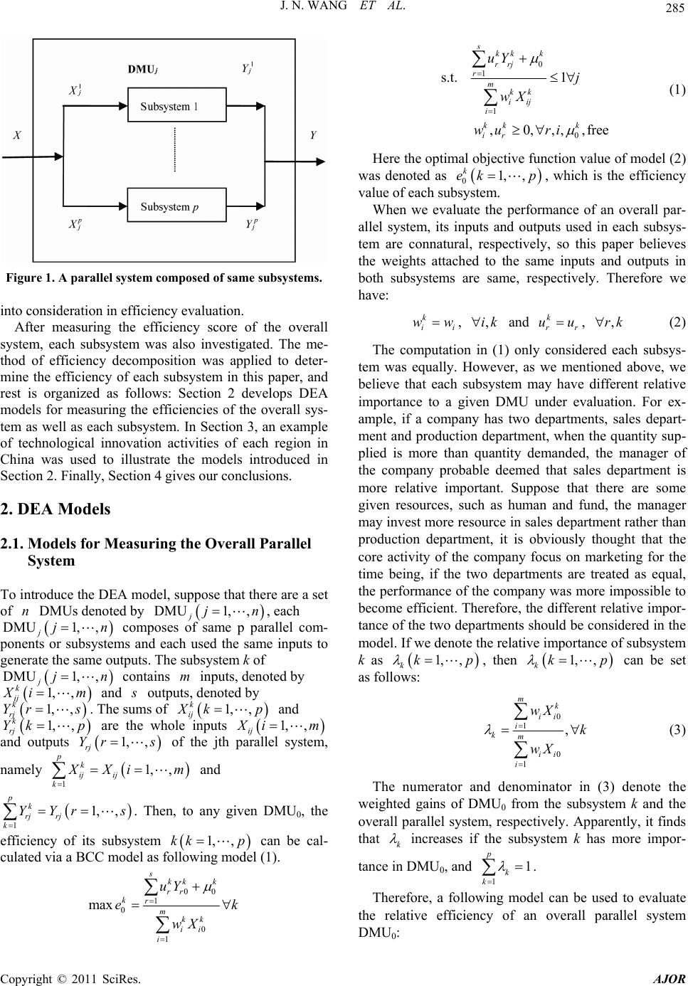

285 J. N. WANG ET AL.
Figure 1. A parallel system composed of same subsystems.
into consideration in efficiency evaluation.
After measuring the efficiency score of the overall
system, each subsystem was also investigated. The me-
thod of efficiency decomposition was applied to deter-
mine the efficiency of each subsystem in this paper, and
rest is organized as follows: Section 2 develops DEA
models for measuring the efficiencies of the overall sys-
tem as well as each subsystem. In Section 3, an example
of technological innovation activities of each region in
China was used to illustrate the models introduced in
Section 2. Finally, Section 4 gives our conclusions.
2. DEA Models
2.1. Models for Measuring the Overall Parallel
System
To introduce the DEA model, suppose that there are a set
of DMUs denoted by , each
composes of same p parallel com-
ponents or subsystems and each used the same inputs to
generate the same outputs. The subsystem k of
contains m inputs, denoted by
n
DMU
DMU
k
ij

DMU1, ,
jjn

n

n

1, ,
jj

1, ,
jj

1, ,
X
im and
s
outputs, denoted by
. The sums of

1, ,
k
rj sYr

1, ,
k
ij
X
k
ij
p and

1, ,
k
rj pYk are the whole inputs

1, ,
X
im
and outputs of the jth parallel system,

1, ,Yrs

rj
namely

1
1, ,
pk
ij ij
k
X
Xi m


 and

1
1, ,
pk
rj rj
k
YYr s




. Then, to any given DMU0, the
efficiency of its subsystem


1, ,kk p can be cal-
culated via a BCC model as following model (1).
00
1
0
0
1
max
skk k
rr
krmkk
ii
i
uY
ek
wX







0
1
1
0
s.t. 1
,0,,,,free
skkk
rrj
rmkk
iij
i
kk k
ir
uY
j
wX
wu ri








 (1)
Here the optimal objective function value of model (2)
was denoted as


01, ,
k
ek p, which is the efficiency
value of each subsystem.
When we evaluate the performance of an overall par-
allel system, its inputs and outputs used in each subsys-
tem are connatural, respectively, so this paper believes
the weights attached to the same inputs and outputs in
both subsystems are same, respectively. Therefore we
have:
k
ii
ww

, ,ik

and , (2)
k
rr
uu,rk
The computation in (1) only considered each subsys-
tem was equally. However, as we mentioned above, we
believe that each subsystem may have different relative
importance to a given DMU under evaluation. For ex-
ample, if a company has two departments, sales depart-
ment and production department, when the quantity sup-
plied is more than quantity demanded, the manager of
the company probable deemed that sales department is
more relative important. Suppose that there are some
given resources, such as human and fund, the manager
may invest more resource in sales department rather than
production department, it is obviously thought that the
core activity of the company focus on marketing for the
time being, if the two departments are treated as equal,
the performance of the company was more impossible to
become efficient. Therefore, the different relative impor-
tance of the two departments should be considered in the
model. If we denote the relative importance of subsystem
k as


1, ,
kk
 p

p, then can be set
as follows:

1, ,
kk
 
0
1
0
1
,
mk
ii
i
km
ii
i
wX
k
wX







(3)
The numerator and denominator in (3) denote the
weighted gains of DMU0 from the subsystem k and the
overall parallel system, respectively. Apparently, it finds
that k

increases if the subsystem k has more impor-
tance in DMU0, and
1
1
p
k
k



.
Therefore, a following model can be used to evaluate
the relative efficiency of an overall parallel system
DMU0:

J. N. WANG ET AL.
286

00
1
0
1
1
0
max
s.t. 1,,
,0,,,,free,
pk
k
k
skk
rrj
rmk
iij
i
k
ir
ee
uY jk
wX
wu rik









 



(4)
In model (4), all the weights attached to the same in-
puts and outputs in both subsystems are replaced by i,
r, as shown in (2). The sets of constraints ensure the
efficiency of each subsystem to all DMUs is not more
than one. The objective function of model (4) is the
weighted objective function of each subsystem based
upon model (1) as follows:
w
u

0
1
pk
k
k
e 


 
0
e (5)
Substitute (1) and (3) into (5), then the objective func-
tion of model (4) can be changed to be:
111
000
11
00
1 1
00
11
00 00
11 1
00
11 1
00 00
11 1
0
1
()
ms
ii rr
pkir
kmm
kii ii
ii
m s
k
0
m
kk
ii ii rr
ii r
mm m
k
ii iiii
ii i
p
s sk
pp rr
rr rk
rmp
ii
i
wX uY
ee
wX wX
wX wX uY
wX wXwX
uY uY
wX



 



 
 
 


 

 
 



 
 
 



p
0
1
m
ii
i
wX



Then the fractional program (4) can be written as fol-
lows:
00
11
0
0
1
0
1
1
0
max
s.t. 1,,
,0,,,,free,.
p sk
rr
rk
m
ii
i
skk
rrj
rmk
iij
i
k
ir
uY
e
wX
uY jk
wX
wu rik











 




(6)
The above program (6) can be converted to the fol-
lowing model by applying the Charnes-Cooper (C-C)
transformation:
000
11
0
11
0
1
0
max
s.t. 0,,
1
,0,,,,free,.
p sk
rr
rk
sm
kk k
rrji ij
ri
m
ii
i
k
ir
eY
YX
X
ri k



 




 

 



jk
(7)
Denote the optimal objective function value of model
(7) as 0 which is the overall parallel efficiency score
of DMU0. It is worth noted that if 0
e
0

, the model
was also established, that is to say the model can be ap-
plied in the case of constant returns to scale.
Definition 1: The overall parallel system of DMU0 is
said to be efficient if 01e

.
Theorem 1: If the overall parallel system of DMU0 is
efficient, then only if its each subsystem is efficient,
namely 01
k
e

, k

.
Proof: First, we prove that is a posi-
tive number which is bigger than 0, but smaller than 1.

1, ,
kk
 

p
First of all, take

as an example, If 10

, then we
obtain 0
r


, r

according to definition (3). Under
this condition, the denominator of (3) is 0, which is
meaningless, so 10


.
If 11


, then we obtain 0,
k

 , for 1k
1
1
p
k
k



. In this case, the denominator of (3) for
0
k


, 1k

 is also 0. Therefore, we have


，01
k
 ,


1, ,kp.
If DMU0 is efficient in overall parallel system (01e

),
then we obtain
1
1
p
kk
k
e 



 based upon (5).
Similarly, suppose the subsystem 1 is non-efficient, in
other words, 1
01e

, Therefore, 1
01
e1

 . However,
according 1
01
2
1
kk
k
ee 

p


and


00, 1
k
e. if
01
k
e

, 1k

,
2
p
kk
k
e 


 obtain the maximum value,
then, 1
01
2
1
p
k
k
e 



, due to and
k
1
1
p
k




1
01
e



, 1
01
2
1
p
k
k
e 



 can be set up only if
1
01e

, if 01
k
e

, 1k

, if holds,
1
01
2
1
p
k
k
e 

 

requires .
1
0
Apparently, it contradicts with the fact that
1e


1, ,
k
ek p
0 is not less than 1. Hence we prove that
the subsystem 1 is efficient ().
1
01e
The similar analysis can be applied to subsystem ,
k

287 J. N. WANG ET AL.

2, ,kp, so 0, . Thus, the theorem has
been completely proven.
1
k
ek
2.2. Models for Measuring Each Subsystem: An
Efficiency Decomposition
Based upon model (7), we can indirectly calculate the
efficiency scores for each subsystem on the use of the
optimal solution. However, the efficiency values of each
subsystem may be non-unique, since the model (7) may
have alternative optimal multipliers. Here we develop
models of efficiency decomposition for each subsystem.
By substitution of each alternative optimal multiplier
which is derived from the model (7), the maximum and
minimum efficiencies values of each subsystem can be
determined. Suppose the maximum and minimum values
of each subsystem of DMU0 can be denoted as 0
k
e and

01, ,
k
ek p, respectively. Then they can be calcu-
lated though the models of following form:
00
1
1
00
11
0
0
, ,
s
rm
i
pk
ii
kk
j
ri








0
1
1
1
ax
, 0,
kd
rr
m
i
rr
j
m
ii
i
ir
uY
wX
uY
wX
wu







0
0
0
minm .
s.t.
1,,
,free,.
kk
rr
k
ii
s
rk
s
r
k
k
uY
ek
wX
e
jk
k











(8)
where 0 is the optimal objective function value of
model (7), and the first constraint ensures that the overall
parallel system maintains its efficiency score invariant.
Similarly, the non-linear program (8) can also be con-
verted into a linear program via C-C transformation as
follows:
e
000
1
00
11
0
11
0
, ,
s
r
k
sm
kk
ri
eY
Y
ri








0 0
1
1
minma .
s.t. 0
0,,
1
,,free,.
k k
rr
p sm
i i
i
k
i ij
m
i
k
k
YeX
Xjk
k












0
x
0,
kd
rr
rk
rr j
k
ii
ir
X







(9)
To distinguish the objective function value in model
(1), here we denote kd
o
e

as objective function value.
Denote the maximum and minimum objective function
values as 0
k
e and


01, ,
k
ek p which can work out
by the model (8). Therefore, the efficiency of each sub-
system k can be determined in an interval

00
,1,,
kk
ee kp


 . If 00
kk
ee, is satisfied, then k
we can conclude that subsystem k has a unique efficiency
value.
Theorem 2: If the overall parallel system of DMU0 is
efficient, then 00 1
kk
ee

, k
Proof: In the Theorem 1 which has proved an overall
parallel system of DMU0 is efficient if and only if its
each subsystem is efficient, namely 0, 1
k
ek

.That is
to say the subsystem has a unique solution equals to 1,
thus, the maximum and minimum efficiencies was only
identified, namely 00
1
kk
ee

, . Then the Theorem k
2 has proved.
2.3. Numerical Example
Here we use the example of Yang et al. (2000), the data
is shown in Table 1. There are 4 DMUs and each has
two subsystems which use single input to generate single
output. Then we use the above models to calculate the
efficiency values for each DMU as well as their each
subsystem, the results are gave in Table 2, in addition,
the third column of Table 2 is the results of the overall
efficiency values for four DMUs when using YMK
model. It can be seen that the efficiency values which are
calculated by two kinds of models are different though
the comparison, however, the common point is both the
results reveal that only DMU 4 is efficient when evalu-
ating the overall system, this proved that two models
have discriminated the most effective DMU. Meanwhile,
Table 1. Data of an example.
Input Output
DMUSubsystem 1Subsystem 2 Subsystem 1 Subsystem 2
1 1 3 1 2
2 2 1 1 1
3 1 3 2 2
4 1 1 3 2

J. N. WANG ET AL.
288
Table 2. Efficiency values of the example.
DMU The overall efficiency value
(model 7)
The overall efficiency value
(YMK model)
The efficiency value of
subsystem 1
The efficiency value of
subsystem 2
1 0.5 0.33 1 0.3333
2 0.6667 0.5 0.5 1
3 0.5 0.667 1 0.3333
4 1 1 1 1
based upon models of efficiency decomposition, each
subsystem was proved that they have unique solution.
The result of DMU 4 illustrates the Theorem 1 as it
shows that the efficiency value of each subsystem is 1. In
addition, for other three inefficient DMUs, only one of
their subsystems is efficient, this brings about monolithic
inefficient. Thus, taking internal structure of the DMU
into consideration is necessary for efficiency evaluation
of the overall system. Besides, take DMU 1 as an exam-
ple, subsystem 2 is considered more important as the
majority of the inputs are allocated to it, if we don not
take the importance of subsystem 2 into consideration,
the efficiency value of subsystem 2 is more than 0.3333.
As subsystem 2 is non-effective, the decision maker
should transfer some inputs to subsystem 1 for improv-
ing the overall performance.
3. Application to Technological Innovation
Organization of Each Region in China
China has an increasing development in the area of tech-
nology since the economic reform in 1978, and these
technological activities have a great contribution to the
economic growth and social development. However,
each province in china demonstrated different efficien-
cies in technological innovation activities. Zhong et al.
(2010) utilize (DEA) models to evaluate the relative effi-
ciencies of 30 regions in China, they indicated that tech-
nological innovation development was unbalance in each
region. In this paper, we believe that the major techno-
logical innovation department of each province includes
three portions: R & D (Research and Development) In-
stitutions, Large & Medium-sized Enterprises and Insti-
tutions of Higher Education. They were considered as a
parallel structure as we described before.
3.1. Selection of Inputs and Outputs and Data
Many different inputs and outputs indices were selected
to evaluate the technological innovation activity. How-
ever, it is well known that the discrimination power of
DEA models will be much weakened if too many inputs
or outputs indicators are used [17], we should chose the
factors that can fully characterize the impact on the per-
formance of technological innovation activity. Zhong [18]
used R & D expenditure and Full-time equivalent of R &
D personnel as inputs and Patent applications, the sales
revenue of new products and the profit of primary busi-
ness as outputs, nevertheless, according to Griliches [19],
Ahuja and Katila [20], R & D expenditure and R & D
personnel, Patent applications and the sales revenue of
new products are the most important inputs and outputs
of technological innovation activity, respectively. In this
paper, the two kinds of core inputs, R & D expenditure
and R & D personnel, were represent by Intramural Ex-
penditure on R & D (: 1000 RMB$) and Full-time equi-
valent of R & D (: man-year) personnel, respectively.
The number of Patent granted (: item) is more appropri-
ate to reflect the outputs of technological innovation ac-
tivity, the sales revenue of new products (: 1000 RMB$),
an index that directly measures product innovation, re-
fers to the sales revenue achieved from sales of new
products in the reporting year. Thus, we have two inputs
and two outputs.
The data we used are 30 regions of China in 2008 with
an exception of Tibet, because of the missing statistical
data. The data is obtained from the China Statistical
Yearbook 2009 and China Statistical Yearbook on sci-
ence and technology 2009. So we omited here.
3.2. Improvement with the Model
Noted that data of outputs, we could not acquire the pre-
cise outputs values to each organization in each province.
Actually in China, the outputs of the technological inno-
vation derive from the combination among these three
organizations. However, in the daily management, each
organization operated independently. The school com-
mits itself to achieve theoretical innovation and break-
through of key technologies, R & D institutions trans-
form the scientific research achievements into products,
the enterprise yields and sales the products and then
gains profit. This indicated that the output of the techno-
logical innovation is an outcome of three organizations.

J. N. WANG ET AL. 289

Y
j
Thus, we give the whole outputs data.
To solve this problem, we assumed that the overall
outputs are divided into three portions to
each organization.

1, 2
ij
Yi
1
ij ij
YY   , and
(10)
2
ij ij
Y  

31
ij ij
YY   
Based upon model (7), by substituting (10) into (7),
then the overall parallel system can be evaluated by fol-
lowing model:


123
00000
1
11
0
11
22
0
11
33
0
11
123
000
1
max
s.t. 0,
0,
10,
1
0,,
s
rr
r
sm
rrji ij
ri
sm
rrji ij
ri
sm
rrjiij
ri
m
iiii
i
eY
YXj
YXj
YX
XXX

 
 
 








 
 
 
 







0
11
,0,,,,free,.
k
ir ri k

 
 

(11)
The above model (11) is a non-linear programming, let
π
rr

 , rr

 , then we can convert it to a
linear programming as follows:

123
0000 0
1
11
0
11
22
0
11
33
0
11 1 1
123
000
1
max
π0,
0,
π0,
1
s
rr
r
sm
rrji ij
ri
sm
rrji ij
ri
sssm
rrjrrjrrji ij
rrr i
m
ii i i
i
eY
YX j
YX j
YYYX
XXX














 





123
000
π;,
,,π,0,, ,,,,free
rrrr
irr r
r
ri

 


j
(12)
By solving model (12), the efficiency value of the
overall system can be obtained. Similarly, we applied the
same method to the models for measuring the efficiency
of each subsystem. The linear programming is showed in
model (13).
000
1
maxmin,1, 2, 3
s
kkk
rr
r
eY k 



11
0
11
22
0
11
33
0
11 11
0
1
123
000 0 00
11
π0,
0,
π0,
1,1,2, 3
0
π;,
,,π,
sm
rrji ij
ri
sm
rrji ij
ri
sssm
rrjrrjrrji ij
rrr i
mk
ii
i
sm
rri i
ri
rrrr
ir rr
YX j
YX j
YYYX
Xk
Ye X
uu r
wu















j











0
0,,,, free,1, 2,3
k
ri k  

(14)
3.3. Results
Based upon the data, we applied model (12) to evaluate
the overall efficiencies of technological innovation in
each region, the results are shown in the second column
of the Table 3. The efficiencies of BCC model which did
not take the internal structure into consideration was
shown in the first column for compare. By analyzing the
two computational results, we can find that the BCC ef-
ficiency values are larger than model (12), this is due to
the model (12) has strong restriction which each techno-
logical innovation organization are compared, rather than
compared only with region. While using BCC model for
measuring, there are seven efficient regions which are
Tianjin, Jilin, Shanghai, Jiangsu, Zhejiang, Guangdong
and Hainan. However, five of them are no longer effi-
cient in our evaluating method, only two regions are
keep efficient, they are Zhejiang and Guangdong, for
these five regions, Jilin has the greatest impact, as we
can see its efficiency value is only 0.6736 when we take
each technological innovation organization into account.
In addition, for other inefficient regions, Shangxi has the
smallest efficiency value, this is same as the conclusion
which can be given by using BCC model, besides, the
efficiency value of Qinghai has the maximum reduction,
as the value decrease 0.3067, and the most possible rea-
son may be the irrational resource allocation of each or-
ganization.
Based upon model (13), the efficiency decomposition
results have shown in the Table 4. The last three col-
umns are the maximum and minimum efficiency values
of each agency, respectively. From the table, we noted
the range that the efficiency values change is extremely
small, and the maximum deviations are only 0.0086
(Liaoning) 0.0109 (Sichuan), 0.0493 (Hunan) in each
organization, respectively. Thus we can conclude that the
ajority of the regions have a unique efficiency value m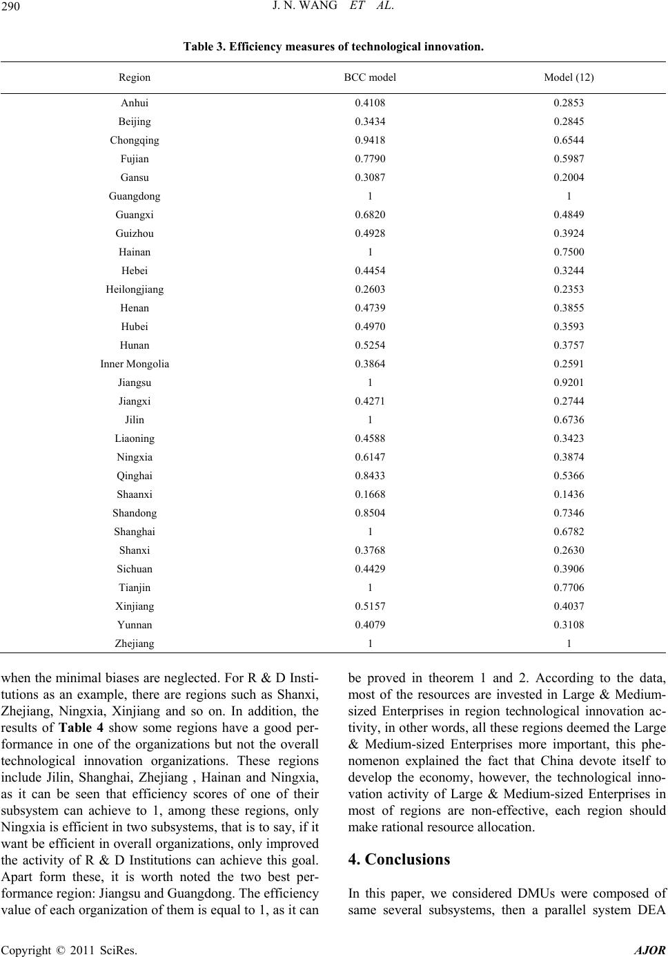

J. N. WANG ET AL.
290
Table 3. Efficiency measures of technological innovation.
Region BCC model Model (12)
Anhui 0.4108 0.2853
Beijing 0.3434 0.2845
Chongqing 0.9418 0.6544
Fujian 0.7790 0.5987
Gansu 0.3087 0.2004
Guangdong 1 1
Guangxi 0.6820 0.4849
Guizhou 0.4928 0.3924
Hainan 1 0.7500
Hebei 0.4454 0.3244
Heilongjiang 0.2603 0.2353
Henan 0.4739 0.3855
Hubei 0.4970 0.3593
Hunan 0.5254 0.3757
Inner Mongolia 0.3864 0.2591
Jiangsu 1 0.9201
Jiangxi 0.4271 0.2744
Jilin 1 0.6736
Liaoning 0.4588 0.3423
Ningxia 0.6147 0.3874
Qinghai 0.8433 0.5366
Shaanxi 0.1668 0.1436
Shandong 0.8504 0.7346
Shanghai 1 0.6782
Shanxi 0.3768 0.2630
Sichuan 0.4429 0.3906
Tianjin 1 0.7706
Xinjiang 0.5157 0.4037
Yunnan 0.4079 0.3108
Zhejiang 1 1
when the minimal biases are neglected. For R & D Insti-
tutions as an example, there are regions such as Shanxi,
Zhejiang, Ningxia, Xinjiang and so on. In addition, the
results of Table 4 show some regions have a good per-
formance in one of the organizations but not the overall
technological innovation organizations. These regions
include Jilin, Shanghai, Zhejiang , Hainan and Ningxia,
as it can be seen that efficiency scores of one of their
subsystem can achieve to 1, among these regions, only
Ningxia is efficient in two subsystems, that is to say, if it
want be efficient in overall organizations, only improved
the activity of R & D Institutions can achieve this goal.
Apart form these, it is worth noted the two best per-
formance region: Jiangsu and Guangdong. The efficiency
value of each organization of them is equal to 1, as it can
be proved in theorem 1 and 2. According to the data,
most of the resources are invested in Large & Medium-
sized Enterprises in region technological innovation ac-
tivity, in other words, all these regions deemed the Large
& Medium-sized Enterprises more important, this phe-
nomenon explained the fact that China devote itself to
develop the economy, however, the technological inno-
vation activity of Large & Medium-sized Enterprises in
most of regions are non-effective, each region should
make rational resource allocation.
4. Conclusions
In this paper, we considered DMUs were composed of
same several subsystems, then a parallel system DEA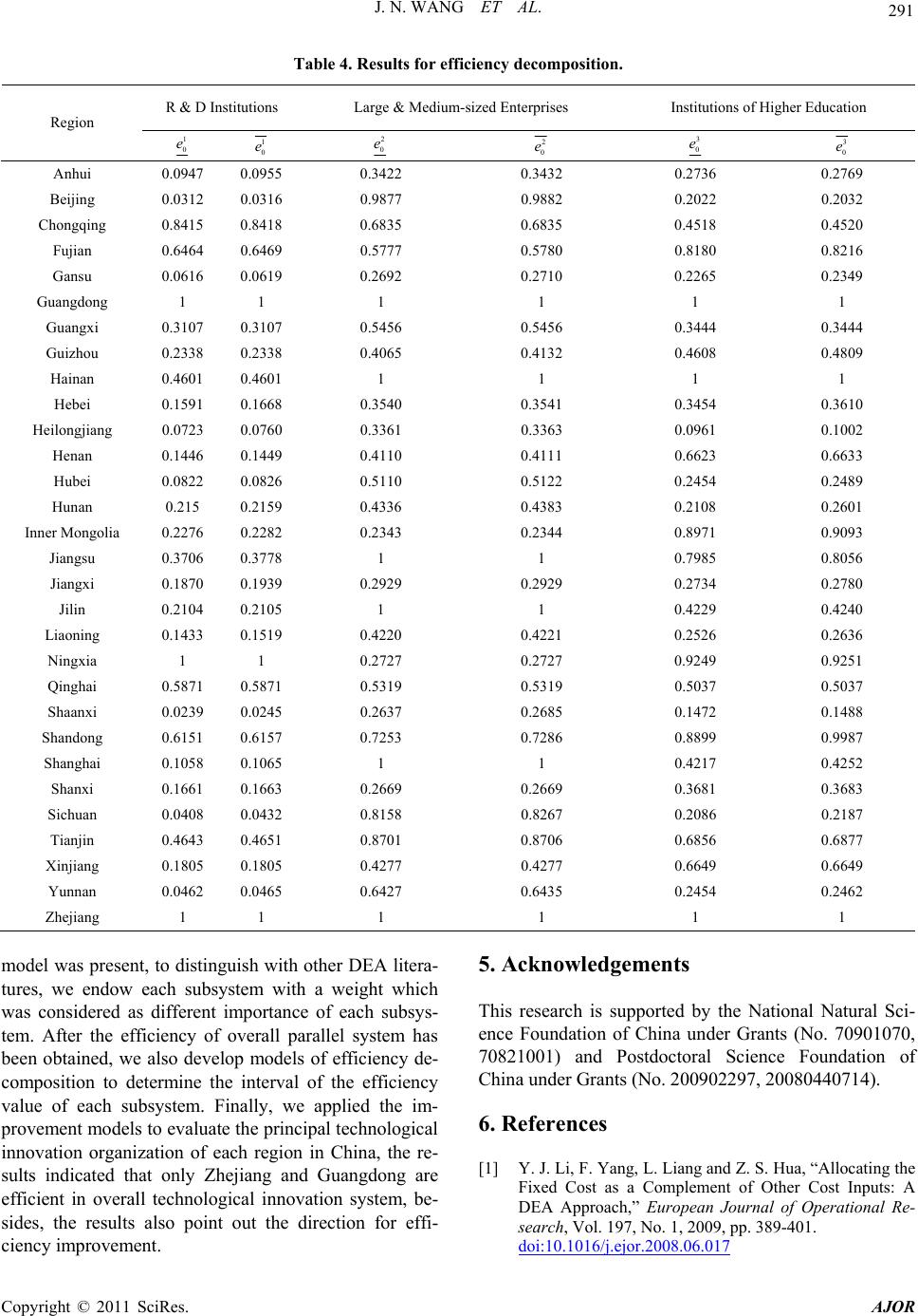

291 J. N. WANG ET AL.
Table 4. Results for efficiency decomposition.
R & D Institutions Large & Medium-sized Enterprises Institutions of Higher Education
Region
1
0
e 1
0
e 2
0
e 2
0
e 3
0
e 3
0
e
Anhui 0.0947 0.0955 0.3422 0.3432 0.2736 0.2769
Beijing 0.0312 0.0316 0.9877 0.9882 0.2022 0.2032
Chongqing 0.8415 0.8418 0.6835 0.6835 0.4518 0.4520
Fujian 0.6464 0.6469 0.5777 0.5780 0.8180 0.8216
Gansu 0.0616 0.0619 0.2692 0.2710 0.2265 0.2349
Guangdong 1 1 1 1 1 1
Guangxi 0.3107 0.3107 0.5456 0.5456 0.3444 0.3444
Guizhou 0.2338 0.2338 0.4065 0.4132 0.4608 0.4809
Hainan 0.4601 0.4601 1 1 1 1
Hebei 0.1591 0.1668 0.3540 0.3541 0.3454 0.3610
Heilongjiang 0.0723 0.0760 0.3361 0.3363 0.0961 0.1002
Henan 0.1446 0.1449 0.4110 0.4111 0.6623 0.6633
Hubei 0.0822 0.0826 0.5110 0.5122 0.2454 0.2489
Hunan 0.215 0.2159 0.4336 0.4383 0.2108 0.2601
Inner Mongolia 0.2276 0.2282 0.2343 0.2344 0.8971 0.9093
Jiangsu 0.3706 0.3778 1 1 0.7985 0.8056
Jiangxi 0.1870 0.1939 0.2929 0.2929 0.2734 0.2780
Jilin 0.2104 0.2105 1 1 0.4229 0.4240
Liaoning 0.1433 0.1519 0.4220 0.4221 0.2526 0.2636
Ningxia 1 1 0.2727 0.2727 0.9249 0.9251
Qinghai 0.5871 0.5871 0.5319 0.5319 0.5037 0.5037
Shaanxi 0.0239 0.0245 0.2637 0.2685 0.1472 0.1488
Shandong 0.6151 0.6157 0.7253 0.7286 0.8899 0.9987
Shanghai 0.1058 0.1065 1 1 0.4217 0.4252
Shanxi 0.1661 0.1663 0.2669 0.2669 0.3681 0.3683
Sichuan 0.0408 0.0432 0.8158 0.8267 0.2086 0.2187
Tianjin 0.4643 0.4651 0.8701 0.8706 0.6856 0.6877
Xinjiang 0.1805 0.1805 0.4277 0.4277 0.6649 0.6649
Yunnan 0.0462 0.0465 0.6427 0.6435 0.2454 0.2462
Zhejiang 1 1 1 1 1 1
model was present, to distinguish with other DEA litera-
tures, we endow each subsystem with a weight which
was considered as different importance of each subsys-
tem. After the efficiency of overall parallel system has
been obtained, we also develop models of efficiency de-
composition to determine the interval of the efficiency
value of each subsystem. Finally, we applied the im-
provement models to evaluate the principal technological
innovation organization of each region in China, the re-
sults indicated that only Zhejiang and Guangdong are
efficient in overall technological innovation system, be-
sides, the results also point out the direction for effi-
ciency improvement.
5. Acknowledgements
This research is supported by the National Natural Sci-
ence Foundation of China under Grants (No. 70901070,
70821001) and Postdoctoral Science Foundation of
China under Grants (No. 200902297, 20080440714).
6. References
[1] Y. J. Li, F. Yang, L. Liang and Z. S. Hua, “Allocating the
Fixed Cost as a Complement of Other Cost Inputs: A
DEA Approach,” European Journal of Operational Re-
search, Vol. 197, No. 1, 2009, pp. 389-401.
doi:10.1016/j.ejor.2008.06.017

J. N. WANG ET AL.
292
[2] A. Charnes, W. W. Cooper and E. Rhodes, “Measuring
the Efficiency of Decision Making Units,” European
Journal of Operational Research, Vol. 2, No. 6, 1978, pp.
429-444. doi:10.1016/0377-2217(78)90138-8
[3] R. D. Banker, A. Charnes and W. W. Cooper, “Some
Models for Estimating Technical and Scale Inefficiencies
in Data Envelopment Analysis,” Management Science,
Vol. 30, No. 9, 1984, pp. 1078-1092.
doi:10.1287/mnsc.30.9.1078
[4] R. Färe and S. Grosskopf, “A Nonparametric Cost Ap-
proach to Scale Efficiency,” Journal of Economics, Vol.
87, No. 4, 1985, pp. 594-604.
[5] L. M. Seiford and R. M. Thrall, “Resent Development in
DEA—The Mathematical Programming Approach to
Frontier Analysis,” Journal of Economics, Vol. 46, No.
1-2, 1990, pp. 7-38.
[6] C. Kao and S. N. Hwang, “Efficiency Decomposition in
Two-Stage Data Envelopment Analysis: An Application
to Non-Life Insurance Companies in Taiwan,” European
Journal of Operational Research, Vol. 185, No. 1, 2008,
pp. 418-429. doi:10.1016/j.ejor.2006.11.041
[7] L. Liang, W. D. Cook and J. Zhu, “DEA Models for
Two-Stage Processes: Game Approach and Efficiency
Decomposition,” Naval Research Logistics, Vol. 55, No.
7, 2008, pp. 643-653. doi:10.1002/nav.20308
[8] Y. Chen, J. Du, H. D. Sherman and J. Zhu, “DEA Model
with Shared Resources and Efficiency Decomposition,”
European Journal of Operational Research, Vol. 207, No.
1, 2010, pp. 339-349.
[9] Y. Zha and L. Liang, “Two-Stage Cooperation Model
with Input Freely Distributed among the Stages,” Euro-
pean Journal of Operational Research, Vol. 205, No. 2,
2010, pp. 332-338. doi:10.1016/j.ejor.2010.01.010
[10] R. Färe and S. Grosskopf, “Network DEA,” Socio-Eco-
nomic Planning Science, Vol. 34, No. 1, 2000, pp. 35-49.
doi:10.1016/S0038-0121(99)00012-9
[11] H. F. Lewis and T. R. Sexton, “Network DEA: Efficiency
Analysis of Organizations with Complex Internal Struc-
ture,” Computers and Operations Research, Vol. 31, No.
9, 2004, pp. 1365-1410.
doi:10.1016/S0305-0548(03)00095-9
[12] K. Tone and M. Tsutsui, “Network DEA: A Slacks-Based
Measure Approach,” European Journal of Operational
Research, Vol. 197, No. 1, 2009, pp. 243-252.
doi:10.1016/j.ejor.2008.05.027
[13] R. Färe and D. Primont, “Efficiency Measures for Multi-
plant Firms,” Operations Research Letters, Vol. 3, No. 5,
1984, pp. 257-260. doi:10.1016/0167-6377(84)90057-9
[14] Y. S. Yang, B. J. Ma and M. Koike, “Efficiency-Mea-
suring DEA Model for Production System with k Inde-
pendent Subsystems,” Journal of the Operations Re-
search Society of Japan, Vol. 43, No. 3, 2000, pp. 343-
353.
[15] L. Castelli, R. Pesenti and W. Ukovich, “DEA-Like Mod-
els for the Efficiency Evaluation of Hierarchically Struc-
tured Units,” European Journal of Operational Research,
Vol. 154, No. 2, 2004, pp. 465-476.
doi:10.1016/S0377-2217(03)00182-6
[16] C. Kao, “Efficiency Measurement for Parallel Production
Systems,” European Journal of Operational Research,
Vol. 196, No. 3, 2009, pp. 1107-1112.
doi:10.1016/j.ejor.2008.04.020
[17] W. Meng, D. Q. Zhang, L. Qi and W. B. Liu, “Two-Level
DEA Approached in Research Evaluation,” Omega, Vol.
36, No. 6, 2008, pp. 950-957.
doi:10.1016/j.omega.2007.12.005
[18] W. Zhong, W. Yuan, S. X. Li and Z. M. Huang, “The
Performance Evaluation of Regional R&D Investments in
China: An Application of DEA Based on the First Offi-
cial China Economic Census Data,” Omega, Vol. 39, No.
4, 2011, pp. 447-455.
doi:10.1016/j.omega.2010.09.004
[19] Z. Griliches, “Patents Statistics as Economic Indicators:
A Survey,” Journal of Economic Literature, Vol. 28, No.
4, 1990, pp. 1661-1707.
[20] G. Ahuja and R. Karila, “Technological Acquisition and
the Innovation Performance of Acquiring Firms: A Lon-
gitudinal Study,” Strategic Management Journal, Vol. 22,
No. 3, 2001, pp. 197-220. doi:10.1002/smj.157