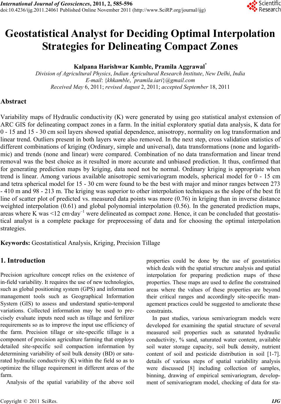International Journal of Geosciences, 2011, 2, 585-596
doi:10.4236/ijg.2011.24061 Published Online November 2011 (http://www.SciRP.org/journal/ijg)
585
Geostatistical Analyst for Deciding Optimal Interpolation
Strategies for Delineating Compact Zones
Kalpana Harishwar Kamble, Pramila Aggrawal*
Division of Agricultural Physics, Indian Agricultural Research Institute, New Delhi, India
Received May 6, 2011; revised August 2, 2011; accepted September 18, 2011
Abstract
Variability maps of Hydraulic conductivity (K) were generated by using geo statistical analyst extension of
ARC GIS for delineating compact zones in a farm. In the initial exploratory spatial data analysis, K data for
0 - 15 and 15 - 30 cm soil layers showed spatial dependence, anisotropy, normality on log transformation and
linear trend. Outliers present in both layers were also removed. In the next step, cross validation statistics of
different combinations of kriging (Ordinary, simple and universal), data transformations (none and logarith-
mic) and trends (none and linear) were compared. Combination of no data transformation and linear trend
removal was the best choice as it resulted in more accurate and unbiased prediction. It thus, confirmed that
for generating prediction maps by kriging, data need not be normal. Ordinary kriging is appropriate when
trend is linear. Among various available anisotropic semivariogram models, spherical model for 0 - 15 cm
and tetra spherical model for 15 - 30 cm were found to be the best with major and minor ranges between 273
- 410 m and 98 - 213 m. The kriging was superior to other interpolation techniques as the slope of the best fit
line of scatter plot of predicted vs. measured data points was more (0.76) in kriging than in inverse distance
weighted interpolation (0.61) and global polynomial interpolation (0.56). In the generated prediction maps,
areas where K was <12 cm·day–1 were delineated as compact zone. Hence, it can be concluded that geostatis-
tical analyst is a complete package for preprocessing of data and for choosing the optimal interpolation
strategies.
Keywords: Geostatistical Analysis, Kriging, Precision Tillage
1. Introduction
Precision agriculture concept relies on the existence of
in-field variability. It requires the use of new technologies,
such as global positioning system (GPS) and information
management tools such as Geographical Information
System (GIS) to assess and understand spatio-temporal
variations. Collected information may be used to pre-
cisely evaluate inputs need such as tillage and fertilizer
requirements so as to improve the input use efficiency of
the farm. Precision tillage or site-specific tillage is a
component of precision agriculture farming that employs
detailed site-specific soil compaction information by
determining variability of soil bulk density (BD) or satu-
rated hydraulic conductivity (K) within the field so as to
optimize the tillage requirement in different areas of the
farm.
Analysis of the spatial variability of the above soil
properties could be done by the use of geostatistics
which deals with the spatial structure analysis and spatial
interpolation for preparing prediction maps of these
properties. These maps are used to define the constrained
areas where the values of these properties are beyond
their critical ranges and accordingly site-specific man-
agement practices could be suggested to ameliorate these
constraints.
In past studies, various semivariogram models were
developed for examining the spatial structure of several
measured soil properties such as saturated hydraulic
conductivity, % sand, saturated water content, available
soil water storage capacity, soil bulk density, nutrient
content of soil and pesticide distribution in soil [1-7].
details of various steps of spatial variability analysis
were discussed [8] including collection of samples,
binning, drawing of empirical semivariogram, develop-
ment of semivariogram model, checking of data for sta-

K. H. KAMBLE ET AL.
586
tionarity, analysis of data for presence or absence of
trend or drift, neighborhood search strategy, different
forms of kriging and their applications under different
situations.
In most of the recent softwares developed for prepar-
ing kriged maps of properties, information about their
spatial structure (semivariogram models) are required in
the input files. Hence spatial structure analysis should be
carried out carefully for preparing semivariogram models.
In softwares like surfer, S+ SpatialStats, GEOEAS (Geo-
statistical Environmental Assessment Software), GS+ etc,
semivariogram models developed are isotropic and there
is limited provision for checking the data for normality,
trend, outliers and anisotropy. In one such study on spa-
tial variation of soil properties of a farm [9], data of vari-
ous properties were not explored for normality, presence
of outliers, anisotropy and presence of trend which were
essential for checking the stationarity. Kriging is not ap-
propriate without removing the cause of nonstationarity
in data. Hence the range of BD as computed were 1053
m and they concluded that their BD and organic carbon
content data showed large amount of nugget variation,
whereas few earlier studies [8,10-11] reported relatively
less range and strong to medium spatial dependence of
these soil properties. Similarly, in another study [12],
stationarity in data was not checked and soil properties
were presumed to be isotropic in nature as GS+ software
was used to determine the spatial structure and thus it
was reported that BD data in their field study was spa-
tially uncorrelated.
Again in one earlier study [11], data for normality and
trend were explored and omnidirectional semivariogram
models were developed by using S+ Spatial Stats soft-
ware, which do not have options about presenting ani-
sotropic nature of semivariogram
With the introduction of Geostatistical Analyst exten-
sion in ArcGIS, it is now possible to carry out explora-
tory spatial data analysis followed by spatial structure
analysis for preparing semivariogram models which can
be used for interpolating data at unvisited sites by choos-
ing appropriate kriging techniques. A distinctive feature
of this statistical package is that it is fully integrated into
the ArcGIS environment, so there is no need to use other
software for preprocessing, statistical analysis and inter-
polation.
Hence, the present study was conducted with the ob-
jective to demonstrate the step by step use of geostatisti-
cal analyst extension of ArcGIS 9.2 for preparing kriged
maps of saturated hydraulic conductivity of soils of IARI
farm for delineation of compact zones.
2. Material and Methods
The study was conducted after the harvest of rainy sea-
son crop at Indian Agricultural Research Institute farm,
New Delhi, India. The study area was in main block of
IARI farm, situated between 77°8'45'' to 77°10'30''E and
28°37'15'' to 28°39'00''N (Figure 1) and had semiarid
climate. 98 sampling points were selected on a rectangu-
lar grid at 100 m × 70 m interval. Land uses were pre-
dominantly maize-wheat and maize-mustard. The soils
(Typic Ustrocrepts) had sandy loam texture.
For determination of K by constant head method, at
each site a core auger of 5 cm diameter was used to take
triplicate soil samples from 0 - 15 and 15 - 30 cm soil
depths.
3. Geospatial Analysis
Drawing of prediction maps of hydraulic conductivity
parameter using Geostatistical Analyst, involved three
key steps [13] :
1) Exploratory spatial data analysis
2) Spatial Structural analysis
3) Surface prediction and assessment of results
3.1. Exploratory Spatial Data Analysis
The boundary shape file of IARI farm along with sam-
pling shape file (point data) were added as layers to
ArcMap. Exploratory Spatial Data Analysis (ESDA)
involves exploring the distribution of the data, looking
for outliers, trends and examining spatial autocorrelation.
Each ESDA tool provides a different view of the data
and is displayed in a separate window. The different
Tools of ESDA are Histogram, Voronoi Map, Trend
Analysis, Semivariogram/Covariance Cloud. Views un-
der all tools interact with one another and with the Arc-
Map map.
3.1.1. Histogram Tool
1) For examining normal distribution: Several meth-
ods in the Geostatistical Analyst require that the data
should be normally distributed. The tool displays the
frequency distribution for the dataset and calculates
summary statistics. For normally distributed data (a bell-
shaped curve), the mean and median should be similar,
the skewness should be near zero, and the kurtosis
should be near 3. If the data is highly skewed, then linear,
box-cox or logarithmic techniques should be used to
make data normal.
2) For detecting global outliers: Outliers can have
several detrimental effects on prediction surface includ-
ing effects on semivariogram modeling and the influence
of neighboring values. A global outlier is a measured
sample point that has a very high or a very low value
relative to all of the values in a dataset. The histogram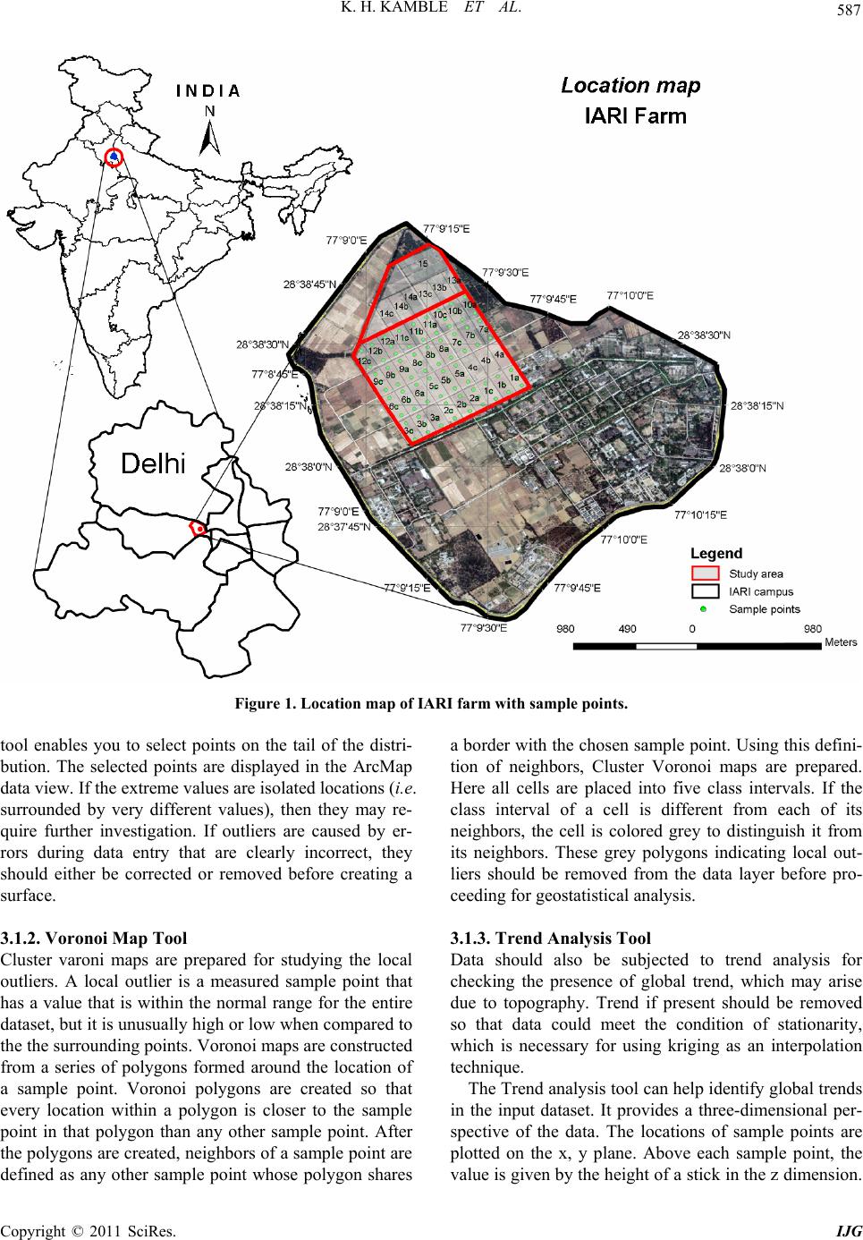

K. H. KAMBLE ET AL.
587
Figure 1. Location map of IARI farm with sample points.
tool enables you to select points on the tail of the distri-
bution. The selected points are displayed in the ArcMap
data view. If the extreme values are isolated locations (i.e.
surrounded by very different values), then they may re-
quire further investigation. If outliers are caused by er-
rors during data entry that are clearly incorrect, they
should either be corrected or removed before creating a
surface.
3.1.2. Voronoi Map Tool
Cluster varoni maps are prepared for studying the local
outliers. A local outlier is a measured sample point that
has a value that is within the normal range for the entire
dataset, but it is unusually high or low when compared to
the the surrounding points. Voronoi maps are constructed
from a series of polygons formed around the location of
a sample point. Voronoi polygons are created so that
every location within a polygon is closer to the sample
point in that polygon than any other sample point. After
the polygons are created, neighbors of a sample point are
defined as any other sample point whose polygon shares
a border with the chosen sample point. Using this defini-
tion of neighbors, Cluster Voronoi maps are prepared.
Here all cells are placed into five class intervals. If the
class interval of a cell is different from each of its
neighbors, the cell is colored grey to distinguish it from
its neighbors. These grey polygons indicating local out-
liers should be removed from the data layer before pro-
ceeding for geostatistical analysis.
3.1.3. Trend Analysis Tool
Data should also be subjected to trend analysis for
checking the presence of global trend, which may arise
due to topography. Trend if present should be removed
so that data could meet the condition of stationarity,
which is necessary for using kriging as an interpolation
technique.
The Trend analysis tool can help identify global trends
in the input dataset. It provides a three-dimensional per-
spective of the data. The locations of sample points are
plotted on the x, y plane. Above each sample point, the
value is given by the height of a stick in the z dimension.

K. H. KAMBLE ET AL.
588
The unique feature of the Trend Analysis tool is that the
values are then projected onto the x, z plane and the y, z
plane as scatter plots. A best fit line (a polynomial) is
drawn through the projected points, which model trends
in specific directions. If the line were flat, this would
indicate that there would be no trend.
3.1.4. Semivariogram/Co variance Cloud
The semivariogram/covariance cloud shows the empiri-
cal semivariogram for all pairs of locations within a data-
set and plots them as a function of the distance between
the two locations. The semivariogram/covariance cloud
can be used to examine the local characteristics of spatial
autocorrelation within a dataset e.g. to check if the sam-
pling interval is well within the range of the spatial cor-
relation between the data points and to explore the direc-
tional influence. It is also examined for presence of out-
liers. Each red dot in the Semivariogram/Covariance
Cloud represents a pair of locations. Since closer loca-
tions should be more alike, in the semivariogram the
close locations (far left on the x-axis) should have small
semivariogram values (low on the y-axis). As the dis-
tance between the pairs of locations increases (move
right on the x-axis), the semivariogram values should
also increase (move up on the y-axis). However, a certain
distance is reached where the cloud flattens out, indicat-
ing that the relationship between the pairs of locations
beyond this distance is no longer correlated. Looking at
the semivariogram, if it appears that some data locations
that are close together (near zero on the x-axis) have a
higher semivariogram value (high on the y-axis) than
others, these pairs of locations should be checked to see
the inaccuracy in data (Local Outliers) and if it is so, in
accurate data points should be removed.
3.2. Spatial Structural Analysis
Steps for use of Geostatistical wizard tool for Investi-
gating sp atial structure (variography):
1) In first step of geostatistical wizard, input data layer
and attribute field on which kriging was to be performed
were selected. Three options of kriging types i.e. Ordi-
nary, Simple and Universal; Two data transformation i.e.
none and log and two trend types i.e none and Linear
were taken. In all 12 combinations were chosen.
2) In the second step of the wizard, for each combina-
tion semivariogram model was developed. For this, the
wizard first determined a good lag size for grouping em-
pirical semivariogram pairs (binning) for reducing their
number. Then it fitted a spherical semivariogram model
(default model) and computed its associated parameter
values namely nugget, range, and partial sill. To actually
account for the directional influences on the semivario-
gram model, directional search tool was used and ani-
sotropical semivariogram model was developed.
3.3. Surface Prediction and Assessment of
Results
In this step of geostatistical wizard, neighborhood search
strategy was decided by taking appropriate shape of
search neighborhood (circular for isotropic and elliptical
for anisotropic data) and dividing it in four quadrants for
avoiding biasness in particular direction. Neighborhood
radius was taken as half of the computed range. Maxi-
mum and minimum number of neighborhood points in
each quadrant were kept between 2 - 5 so as to use a total
of 8 - 20 neighbor points for interpolation.
The Geostatistical Analyst predicted the value at un-
known location by using the equation:
 
1


n
oii
i
Z
sZs
where Z(si) is the measured value at the ith location and
i

is an unknown weight for measured value at the ith
location, o
s
is the prediction location. N is number of
measured points used for estimation. To ensure the pre-
dictor is unbiased for the unknown measurement, the
sum of the weights i

must equal one. These weights
could be computed by solving the ordinary kriging equa-
tions given below:
11 1110
10
= g
or
1
1
110 1

 
 













N
NNN NN
m
Fitted semivariogram models were used for creating Г
matrix and g vectors which then were used for solving
for the kriging weights vector λ by matrix. Summation of
the weight for each measured value times the value
would be the final prediction value for the location.
4. Performing Cross Validation to Assess
Parameter Selections
Cross-validation helps in deciding the model which
makes the best predictions. The calculated statistics serve
as diagnostics that indicate whether decisions on choice
of method of kriging, as well as on choice of transforma-
tion and order of trend decided from ESDA are reason-
able to provide an unbiased and more accurate prediction
of parameter values along with valid prediction standard
errors. Cross-validation tool of geostatistical wizard

K. H. KAMBLE ET AL.
589
gives a scatter plot of predicted vs measured values and a
best fit linear line (green solid line) through it. Higher the
slope of this line (magnitude always <1), nearer it will be
to 1:1 line (black dashed line) which is an indicator of
good prediction choices. If all the data are spatially in-
dependent, best fit line would be horizontal.
For a model that provides unbiased predictions, the
mean of prediction errors should be close to zero. Again
for the correct assessment of the variability and to check
if the prediction standard errors are appropriate and valid,
the root-mean-square prediction error and average stan-
dard prediction error should be similar and the root-mean
square standardized prediction error should be close to 1.
5. Delineation of Compact Zones
For delineation of compaction zones, prediction map of
the best choice i.e. the most suited kriging type, data
transformation, trend type and semivariance model should
be used. Map should be divided into five hydraulic con-
ductivity classes namely 0 - 6, 6 - 12, 12 - 24, 24 - 72
and 72 - 150 cm·day–1 as used in physical rating of soils
[14]. The areas of the map with saturated hydraulic con-
ductivity values <12 cm·day–1 were considered as com-
pact zones.
6. Results
6.1. Exploratory Data Analysis
First of all, histogram tool was used to examine the fre-
quency distribution of data for checking its normality
and presence of outlier (Figure 2 and Table 1). As the
differences between mean and median were 5.04 and
3.13, respectively, for 0 - 15 and 15 - 30 cm layers.
Similarly the skewness values of both layers were 1.52
and 0.78. The above results thus indicated that data were
far away from being normal. But data on log transforma-
tion of for both layers showed normal distribution.
In second step, varoni map tool was used to prepare
cluster varoni map for examining the presence of outliers
which were shown as grey cell polygons. These data
points were highlighted in Arc map and were removed as
shown in Figure 3.
In third step semivariance tool was used for examining
the empirical semivariogram which clearly indicated that
data were spatially correlated. Each red dot in semivario-
gram cloud represents a semi variance value which is the
difference squared between the values of each pair of
location and is plotted on y-axis relative to the distance
separating each pair on the x-axis. Green points on the
Table 1. Summary statistics of measured hydraulic conduc -
tivity data of 0 - 15 and 15 - 30 cm soil layers of farm.
TransformationNone Log
Depth (cm) 0 - 15 15 - 30 0 - 15 15 - 30
Count 72 51 72 51
Min 1.44 2.88 0.36 1.06
Max 109.44 66.24 4.70 4.19
Mean 24.55 21.85 2.78 2.79
Median 19.51 18.72 2.97 2.93
Kurtosis 6.07 2.92 2.95 2.44
Skewness 1.52 0.78 –0.74 –0.54
Std.Dev 20.76 15.33 1.06 0.85
Figure 2. Histogram showing nor mal distribution of no transformation and log transformation of hy draulic conductivity (K)
for depth 0 - 15 cm.
Data 10
2

K. H. KAMBLE ET AL.
590
Figure 3. Show ing the local outliers be ing removed by using
cluster type in voronoi map.
other hand indicates the number of pairs made by a given
point with its neighborhood. It appeared that some data
locations that were close together (near zero on the x-
axis) had very high semivariance values (high on the y-
axis) which indicated the possibility of inaccuracy in
data. i.e. the presence of local outliers. Such local out-
liers (red dots with very high variance at small lag dis-
tances) were highlighted and removed (Figure 4). To
explore for a directional influence in the semivariogram
cloud, search direction tool was used, which indicated
anisotropic nature of data.
In the fourth step, trend Analysis tool was used to
examine if trend is present in both XZ and YZ planes in
different directions by looking at the shapes of both
green and blue lines. For 0 - 15 cm layer, trend in XZ
direction was negligible, where as trend in YZ direction
was linear (Figure 5). For 15 - 30 cm soil layer slight
trend was present in both XZ and YZ directions. Pres-
ence of trend in surface layer in YZ direction was attrib-
uted to 1% - 3% slope in Y direction and no trend be-
cause of slope <0.5% in X direction.
Figure 4. Showingsemivariogram cloud.
Figure 5. Trend showing on projected data of K (0 - 15 cm).

K. H. KAMBLE ET AL.
591
6.2. Geostatistical Wizard for Spatial Structure
Analysis
In Geostatistical wizard, firstly sampling points data layer
(after removing local and global outliers) and attribute
field i.e. HC of 0 - 15 cm layer were selected. Then dif-
ferent combinations of kriging (Ordinary, simple and
universal), data transformations (none and logarithmic)
and trends (none and linear) were taken and their cross
validation statistics were compared (Figure 6). It was
observed that for all types of kriging, with no transfor-
mation of data and without removal trend, predictions
were unbiased as mean of prediction errors was nearer to
zero (0.003 - 0.097) and prediction of standard errors
were appropriate as indicated by the closeness of the
root-mean-square prediction error and average standard
prediction error values (differences in their magnitude
were 0.08 - 0.3). But predictions were not close to meas-
ured values as indicated by appreciable magnitude of
root-mean-square prediction error (nearly 17.4) and also
best fit line was far away from 1:1 line and slope of best
fit line was less (0.47). The results thus described these
choices as not desirable. Again for all kriging types, on
log transformation of data along with no trend removal
option, although the slope of best fit line increased (0.61
- 0.63) as compared to no transformation but the magni-
tude of other cross validation statistical parameters for
deciding the biasness of prediction (higher mean of pre-
diction errors of the order of 2.8 - 2.9) and validity of
estimated prediction errors were not satisfactory (large
differences between root-mean-square prediction error
and average standard prediction error of the order of 12 -
40). Similarly irrespective of kriging type, on log trans-
formation of data and linear trend removal (the choices
suggested by ESDA), the slope of best fit line improved
further but the magnitude of other cross validation pre-
diction error parameters were not indicating these choices
as the suitable ones. However, the combination of no
data transformation and linear trend removal indicated
higher slope of best fitted line (0.55 - 0.77), lower mag-
Figure 6. Comparison of crossvalidation statistics of different kriging methods (ordinary, universal, simple), data transfor-
mations (none, log) and trend types (none, first).

K. H. KAMBLE ET AL.
592
nitude of mean of prediction errors (0 - 0.27), less dif-
ferences (1 - 4) between root-mean-square prediction
error and average standard prediction error. The above
analysis thus indicated combination of no data transfor-
mation and linear trend removal is the best choice as it
resulted in more accurate and unbiased prediction of data.
The above results thus confirm the earlier findings [8,15]
that for drawing prediction maps by kriging, data need
not be normal, but trend if present should be removed in
order to remove the cause of nonstationarity in data be-
fore making predictions.
On comparing the cross validation statistics of all
three methods of kriging (with no data transformation
and linear trend removal), ordinary kriging was found to
be the most suited choice for interpolation. The results
were in agreement with those earlier reported [8] where
it was mentioned that universal is more appropriate when
trend is of higher order. Similar results were obtained
when K data was analysed for 15 - 30 cm soil layer.
After selecting ordinary kriging with no data trans-
formation and removing linear trend, cross validation
statistics of different semivariogram models were also
Table 2. Parameters of different semivar igram models for predicting the spatial structure of hydraulic conductivity of 0 - 15
and 15 - 30 cm soil layer.
Model Nugget (cm·day–1) Major range (m) Minor range (m) Direction Partial sill (cm·day–1)
0 - 15
Circular 0.00 244.62 87.30 18 332.44
Spherical 0.00 273.89 98.28 18 332.46
Tetraspherical 0.00 273.89 104.78 9 329.35
Pentaspherical 0.00 273.89 113.68 9 327.71
Exponential 0.00 273.89 110.42 9 335.99
Gaussian 0.33 224.60 82.25 18 334.19
Rational Quadratic 0.33 273.89 90.50 351 331.94
Hole Effect 108.99 203.15 91.41 333 214.18
K-Bessel 0.00 234.04 85.42 18 335.14
J-Bessel 194.36 273.89 81.49 333 122.89
Stable 0.00 230.25 83.89 18 334.64
15 - 30
Circular 75.14 410.04 183.71 54 160.74
Spherical 65.06 410.04 200.54 54 168.93
Tetraspherical 55.65 410.04 213.74 54 176.86
Pentaspherical 47.03 410.04 225.83 54 184.36
Exponential 0.00 410.04 174.62 54 236.49
Gaussian 102.96 410.04 178.58 54 134.02
Rational Quadratic 0.24 410.04 205.44 54 237.93
Hole Effect 91.34 410.04 309.62 63 127.19
K-Bessel 47.20 217.95 300.32 0 178.96
J-Bessel 97.47 410.04 332.17 63 109.96
Stable 99.29 410.04 179.56 54 137.43

K. H. KAMBLE ET AL.
593
compared to choose the best option (Table 2). Spherical
model for 0 - 15 cm and tetra spherical model for 15 - 30
cm were found to be the best. It was further observed
that for drawing semivariogram, lag size of 23 m along
with 12 number of lags were chosen by wizard as default
choices (Table 3) which were in accordance to the
thumb rule that product of lag size and no of lags (23 ×
12 = 276 m) should be less than half of the maximum
distance between farthest pair of points (nearly 1200 m).
Semivariogram showed anisotropic nature with major
and ranges of 273 m and 410 m and minor range of 98
and 213, respectively, for 0 - 15 and 15 - 30 cm layer.
The superiority of kriging over other interpolation
techniques was obvious as the slopes of best fit line in 4th
power under inverse distance weighted interpolation
(IDW) and global polynomial interpolation (GP) were
0.61 and 0.56 against 0.76 under ordinary kriging (Fig-
ure 7). Besides making more accurate predictions, kriging
Table 3. Comparison of cross validation statistics of different models by Ordinary Kriging with no transformation and first
order trend
Model Mean Root-Mean-Square Average Standard Erro
r
Mean StandardizedRoot-Mean-Square Sta ndardized Regression equation
(K 0 - 15)
Circular 0.19 13.75 17.13 0.0091 0.84 0.763*x + 5.995
Spherical 0.17 13.81 17.28 0.0084 0.84 0.765*x + 5.498
Tetraspherical 0.05 14.64 17.62 0.0017 0.85 0.709*x + 6.652
Pentaspherical 0.08 14.85 17.77 0.0030 0.85 0.693*x + 7.316
Exponential 0.03 14.82 17.81 0.0006 0.85 0.684*x + 7.550
Gaussian 0.14 13.72 17.20 0.0063 0.83 0.753*x + 5.991
Rational Quadratic –0.08 16.10 18.05 –0.0049 0.90 0.573*x + 8.715
Hole Effect 0.46 15.74 17.60 0.0223 0.90 0.675*x + 8.024
K Bessel 0.13 13.74 17.23 0.0058 0.83 0.753*x + 6.006
J Bessel 0.70 15.39 17.76 0.0378 0.88 0.673*x + 7.887
Stable 0.13 13.74 17.21 0.0060 0.83 0.751*x + 5.788
(K 15 - 30)
Circular 0.19 11.10 12.08 0.0135 0.95 0.623*x + 7.341
Spherical 0.27 11.09 11.98 0.0197 0.96 0.648*x + 6.878
Tetraspherical 0.21 10.77 11.91 0.0150 0.95 0.674*x + 6.249
Pentaspherical 0.12 11.51 12.83 0.0091 0.92 0.565*x + 9.634
Exponential 0.25 10.52 12.57 0.0175 0.87 0.674*x + 6.875
Gaussian 0.17 11.58 12.29 0.0119 0.97 0.480*x + 10.153
Rational Quadratic 0.37 10.42 13.04 0.0253 0.83 0.664*x + 7.229
Hole Effect 0.06 12.52 12.91 0.0019 1.00 0.549*x + 9.669
K Bessel 0.17 11.35 12.15 0.0123 0.97 0.575*x + 8.414
J Bessel 0.08 12.36 12.92 0.0035 0.99 0.522*x + 10.585
Stable 0.16 11.39 12.19 0.0110 0.97 0.570*x + 8.529

K. H. KAMBLE ET AL.
594
Figure 7. Comparison of cross validation statistics of different interpolation methods.
also gave prediction error maps of the data.
It was also learned that by increasing the sample size
from 36 to 50 and 50 to 72, prediction improved as indi-
cated by the increased value of slope of best fit line of
scatter plot from 0.29 to 0.45 and from 0.45 to 0.76
(Figure 8). The lesser the number of samples in a given
area means the separation interval between pairs in-
creases and such pairs are representative of variance
structure not the majority of the samples [8]. Since the
area covered for prediction was 72 ha, it could be stated
that at least one sampling point is required per hectare.
Final prediction layers of K for both soil depths were
presented as filled contours with 5 classes (Figure 9).
The area on the prediction map with K value <12
cm·day–1 was delineated as compact area. It was further
analyzed that 41% - 42% of total area was under com-
paction for both layers. Hence instead of carrying out
chiseling in the whole farm, it is required in less than
half of the field, which could result in a saving of 50% of
fuel and time.
7. Conclusions
Geostatistical Analyst has served as a bridge between
geostatistics and GIS. In the other available kriging
softwares, few geostatistical tools have been available,
but only in geostatistical analyst, all tools are available
and also integrated within GIS modeling environments.
The most important feature of such Integration is that
now it is possible to quantify the quality of prediction
surface models by measuring the statistical error of pre-
dicted surfaces. In conclusion it could be stated that geo-
statistical analyst is a complete package for analysis of
spatial variation of a given parameter on field scale and
for assessing the various choices for drawing optimum
and unbiased prediction surfaces.
The above study also suggests that Geostatistical ana-
lyst extension could be used as a tool for interpolation of
data if it the sampling interval of the parameter is less
than half of its major range. Thus its use is limited to
field scale only. Study also indicated the superiority of

K. H. KAMBLE ET AL.
595
Figure 8. Comparison of cross validation statistics of predicted K(0 - 15) data with different number of sampling points.
Figure 9. Prediction maps of K of 0-15 and 15-30 cm soil layers of main block of IARI farm.

K. H. KAMBLE ET AL.
596
Kriging over IDW in terms of more accuracy in predic-
tion as suggested by higher slope of regression line
drawn between observed and predicted points. In order to
improve upon the existing geostatistical analyst exten-
sion, block kriging option should also be included along
with other options of interpolation so that it could be
used for interpolation on regional scale.
8. References
[1] W. A. Jury, “Spatial Variability of Soil Properties”, In: S.
C. Hern and S. M. Melancon, Eds., Vadose Zone Model-
ling of Organic Pollutants, Lewis Publishers, Boca Raton,
1986, pp. 245-269.
[2] A. W. Warrick, D. E. Myers and D. R. Nielsen, “Geosta-
tistical Methods Applied to Soil Science,” In: A. Klute,
Eds., Methods of Soil Analysis, Part I, 2nd Edition, Soil
Science Society of America Book, Madison, 1986, pp.
53-82.
[3] P. Aggarwal and R. P. Gupta, “Two Dimensional Geosta-
tistical Analysis of Soils,” In: R. P. Gupta and B. P.
Gnildyal, Eds., Theory and Practice in Agrophysics
Measurements, Allied Publishers, Buffalo, 1998, pp.
253-263.
[4] I. S. Dahiya, B. Kalta and R. P. Agrawal, “Kriging for
Interpolation through Spatial Variability Analysis of
Data,” In: R. P. Gupta, B. P. Ghildyal, Eds., Theory and
Practice in Agrophysics Measurements, Allied Publishers,
Buffalo, 1998, pp. 242-252.
[5] A. B. McBratney and M. J. Pringle, “Estimating Average
and Proportional Variograms of Soil Properties and Their
Potential use in Precision Farming,” Precision. Agricul-
ture, Vol. 1, No. 2, 1999, pp. 219-236.
doi:10.1023/A:1009995404447
[6] M. Mzuku, R. Khosla, R. Reich, D. Inman, F. Smith and
L. Macdonald, “Spatial Variability of Measured Soil
Properties across Site Specific Management Zones,” Soil
Science. Society of America Journal, Vol. 69, No. 5, 2005,
pp. 1572-1579. doi:10.2136/sssaj2005.0062
[7] A. Sarangi, C. A. Cox and C. A. Madramootoo, “Geosta-
tistical Methods for Prediction of Spatial Variability of
Rainfall in a Mountainous Region,” Transactions of
ASAE, Vol. 48, No. 3, 2005, pp. 943-954.
[8] D. J. Mulla and A. B. McBratney, “Soil Spatial Variabil-
ity,” In: A. W. Warrick, Ed., Soil Physics Companion,
CRC Press, Boca Raton, 2002, pp. 343-370.
[9] P. Santra, U. K. Chopra and D. Chakraborty, “Spatial
Variability of Soil Properties and Its Application in Pre-
dicting Surface Map of Hydraulic Parameters in an Agri-
cultural Farm,” Current Science, Vol. 95, No. 7, 2008, pp.
937-945.
[10] K. Kılıç, E. Özgöz and F. Akba, “Assessment of Spatial
Variability in Penetration Resistance as Related to Some
Soil Physical Properties of Two Fluvents in Turkey,” Soil
Tillage Research, Vol. 76, No. 1, 2004, pp .1-11.
[11] J. Iqbal, J. A. Thomasson , J. N. Jenkins, P. R. Owen and
F. D. Whisler, “Spatial Variability Analysis of Soil Physi-
cal Properties of Alluvial Soils,” Soil Science Society of
America Journal, Vol. 69, No. 4, 2005, pp. 1338-1350.
doi:10.2136/sssaj2004.0154
[12] M. Dufferra, G. W. Jeffrey and R. Weisz, “Spatial Vari-
ability of Southeastern U.S. Coastal Plain Soil Physical
Properties: Implications for Site-Specific Management,”
Geoderma, Vol. 137, No. 3-4, 2007, pp. 327-339.
doi:10.1016/j.geoderma.2006.08.018
[13] J. M. Ver Hoef, K. Krivoruchko and N. Luca, “Using
ARCGIS Geostatistical Analyst,” ESRI, St. Charles, 2001,
pp. 1-306.
[14] R. P. Gupta and I. P. Abrol, “A Study of Some Tillage
Practices for Sustainable Crop Production in India,” Soil
& Tillage Research, Vol. 27, No. 1-4, 1993, pp. 253-273.
doi:10.1016/0167-1987(93)90071-V
[15] K. Johnston, J. M. V. Hoef, K. Krivoruchko and N. Lucas,
“Using Geostatatistical Analyst,” ESRI, St. Charles, 2001,
pp. 1-306.