Applied Mathematics, 2011, 2, 1405-1416
doi:10.4236/am.2011.211199 Published Online November 2011 (http://www.SciRP.org/journal/am)
Prey Predator Fishery Model with Stage Structure in Two
Patchy Marine Aquatic Environment
Mellachervu Naga Srinivas1, Mantripragada Ananata Satya Srinivas2,
Kalyan Das1, Nurul Huda Gazi3
1School of Advanced Sciences, Department of Mathematics, VIT University, Vellore, India
2Department of Mathematics, Jawaharlal Nehru Technological University, Hyderabad, India
3Department of Mathematics, Aliah University, Kolkata, India
Received July 4, 2011; revised August 2, 2011; accepted August 9, 2011
Abstract
In this paper, we propose and analyze a mathematical model to study the dynamics of a fishery resource sys-
tem with stage structure in an aquatic environment that consists of two zones namely unreserved zone (fish-
ing permitted) and reserved zone (fishing is strictly prohibited). In this model we introduce a stage structure
in which predators are split into two kinds as immature predators and mature predators. It is assumed that
immature predators cannot catch the prey and their foods are given by their parents (mature predators). It is
also assumed that the fishing of immature predators prohibited in the unreserved zone and predator species
are not allowed to enter inside the reserved zone. The local and global stability analysis has been specified.
Biological and Bionomical equilibriums of the system are derived. Mathematical formulation of the optimal
harvesting policy is given and its solution is derived in the equilibrium case by using Pontryagin’s maximum
principle.
Keywords: Prey Predator, Stage Structure, Local and Global Stability, Bionomic Equilibrium, Optimal
Harvesting, Pontryagin’s Maximum Principle
1. Introduction
There are numerous studies on the effects of harvesting
on population growth. In the context of Predator-prey
interaction, some studies that treat the populations being
harvested as a homogeneous resource include those of
Brauer and Soudack [1,2], Dai and Tang [3], Myer-
scough et al. [4], Chaudhuri [5] and Leung [6]. For a first
look at the problem of harvesting from a bioeconomic or
control theory point of view, see the works of Clark [7]
and Levin et al. [8]. But they have not considered stage
structure of species. Some of the stage structured models
using time delay were considered by Aiello and Freed-
man [9], Freedman and Gopalsammy [10], Rosen [11],
Fisher and Goh [12], Cushing and Saleem [13], and some
other authors. In general, stage structured models exhibit
much more complicated dynamics than ordinary models.
Bioeconomic modeling of the exploitation of biologi-
cal resources such as fisheries and fore tries has gained
importance in recent years. The techniques and issues
associated with the bioeconomic exploitation of these
resources have been discussed in detail by Clark [7,14].
Since most marine fisheries are essentially multi species
in nature, exploitation of mixed species fisheries has
started to draw attention from researchers. Although nu-
merous models on single species fisheries have so far
appeared in the fishery literature, no fully adequate stud-
ies on multispecies fisheries appear to exist.
It is very difficult to construct a realistic model of a
multispecies community. Even if we succeed in formu-
lating such a model, it is quite likely that the model may
not be analytically tractable. Not every part of the catch
is edible and harvesting harms some of the marine spe-
cies which live on the other species in the sea. Thus the
predator species are likely to become extinct with an in-
discrete increase in the harvesting of prey species. There-
fore, how best to harvest an ecologically or economically
interdependent population in the sense of maximizing the
present value of a stream of revenues from them, while
maintaining ecological balance, is an important optimal
control problem for fisheries.
Clark [14] discussed an optimal equilibrium policy for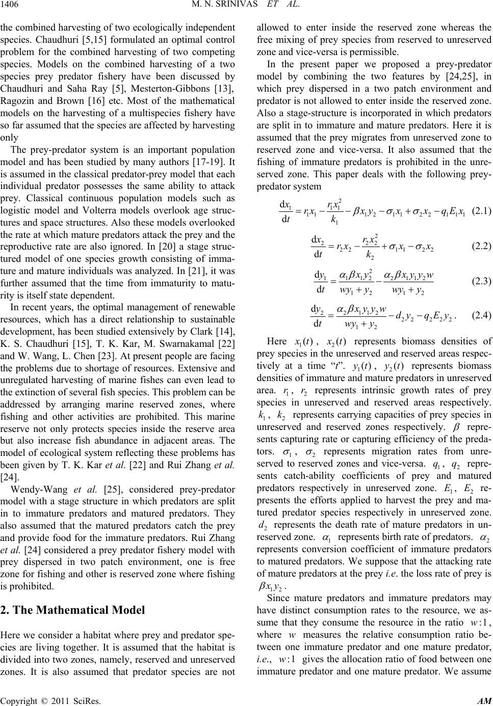

M. N. SRINIVAS ET AL. 1406
the combined harvesting of two ecologically independent
species. Chaudhuri [5,15] formulated an optimal control
problem for the combined harvesting of two competing
species. Models on the combined harvesting of a two
species prey predator fishery have been discussed by
Chaudhuri and Saha Ray [5], Mesterton-Gibbons [13],
Ragozin and Brown [16] etc. Most of the mathematical
models on the harvesting of a multispecies fishery have
so far assumed that the species are affected by harvesting
only
The prey-predator system is an important population
model and has been studied by many authors [17-19]. It
is assumed in the classical predator-prey model that each
individual predator possesses the same ability to attack
prey. Classical continuous population models such as
logistic model and Volterra models overlook age struc-
tures and space structures. Also these models overlooked
the rate at which mature predators attack the prey and the
reproductive rate are also ignored. In [20] a stage struc-
tured model of one species growth consisting of imma-
ture and mature individuals was analyzed. In [21], it was
further assumed that the time from immaturity to matu-
rity is itself state dependent.
In recent years, the optimal management of renewable
resources, which has a direct relationship to sustainable
development, has been studied extensively by Clark [14],
K. S. Chaudhuri [15], T. K. Kar, M. Swarnakamal [22]
and W. Wang, L. Chen [23]. At present people are facing
the problems due to shortage of resources. Extensive and
unregulated harvesting of marine fishes can even lead to
the extinction of several fish species. This problem can be
addressed by arranging marine reserved zones, where
fishing and other activities are prohibited. This marine
reserve not only protects species inside the reserve area
but also increase fish abundance in adjacent areas. The
model of ecological system reflecting these problems has
been given by T. K. Kar et al. [22] and Rui Zhang et al.
[24].
Wendy-Wang et al. [25], considered prey-predator
model with a stage structure in which predators are split
in to immature predators and matured predators. They
also assumed that the matured predators catch the prey
and provide food for the immature predators. Rui Zhang
et al. [24] considered a prey predator fishery model with
prey dispersed in two patch environment, one is free
zone for fishing and other is reserved zone where fishing
is prohibited.
2. The Mathematical Model
Here we consider a habitat where prey and predator spe-
cies are living together. It is assumed that the habitat is
divided into two zones, namely, reserved and unreserved
zones. It is also assumed that predator species are not
allowed to enter inside the reserved zone whereas the
free mixing of prey species from reserved to unreserved
zone and vice-versa is permissible.
In the present paper we proposed a prey-predator
model by combining the two features by [24,25], in
which prey dispersed in a two patch environment and
predator is not allowed to enter inside the reserved zone.
Also a stage-structure is incorporated in which predators
are split in to immature and mature predators. Here it is
assumed that the prey migrates from unreserved zone to
reserved zone and vice-versa. It also assumed that the
fishing of immature predators is prohibited in the unre-
served zone. This paper deals with the following prey-
predator system
2
111
111 2112 2111
1
d
d
xrx
rx xyxxqE
tk
  x (2.1)
2
222
2211 22
2
d
d
xrx
rxx x
tk
  (2.2)
2
11122112
12 12
d
d
yxy xyy
twyy wyy
 


w
(2.3)
22112
222 22
12
d
d



yxyyw
dy qEy
twyy . (2.4)
Here 1()x t, 2()xt represents biomass densities of
prey species in the unreserved and reserved areas respec-
tively at a time “t”. 1, 2 represents biomass
densities of immature and mature predators in unreserved
area. 1, 2 represents intrinsic growth rates of prey
species in unreserved and reserved areas respectively.
1, 2 represents carrying capacities of prey species in
unreserved and reserved zones respectively.
()yt ()yt
r
k
r
k
 repre-
sents capturing rate or capturing efficiency of the preda-
tors. 1
 , 2  represents migration rates from unre-
served to reserved zones and vice-versa. 1, 2 repre-
sents catch-ability coefficients of prey and matured
predators respectively in unreserved zone. 1, 2 re-
presents the efforts applied to harvest the prey and ma-
tured predator species respectively in unreserved zone.
2 represents the death rate of mature predators in un-
reserved zone. 1
q q
E E
d
 represents birth rate of predators. 2 
represents conversion coefficient of immature predators
to matured predators. We suppose that the attacking rate
of mature predators at the prey i.e. the loss rate of prey is
12
x y  .
Since mature predators and immature predators may
have distinct consumption rates to the resource, we as-
sume that they consume the resource in the ratio ,
wher e measures the relative consumption ratio be-
tween one immature predator and one mature predator,
i.e., gives the allocation ratio of food between one
immature predator and one mature predator. We assume
:1w
w
:1w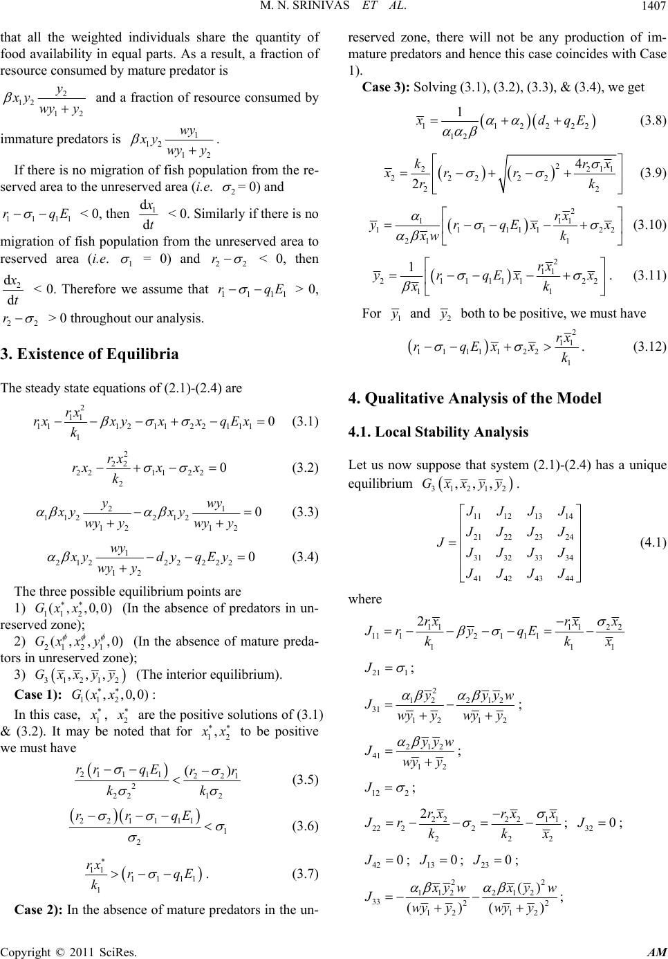

M. N. SRINIVAS ET AL.1407
that all the weighted individuals share the quantity of
food availability in equal parts. As a result, a fraction of
resource consumed by mature predator is
2
12
12
y
xy wy y 
 and a fraction of resource consumed by
immature predators is 1
12
12
wy
xy wy y 
.
If there is no migration of fish population from the re-
served area to the unreserved area (i.e. 2

= 0) and
111
rq
1
E

 < 0, then 1
d
d
x
t < 0. Similarly if there is no
migration of fish population from the unreserved area to
reserved area (i.e. 1

= 0) and 2 r2

 < 0, then
2
d
d
x
t < 0. Therefore we assume that 11
r1 q
1
E

 > 0,
2
r2

 > 0 throughout our analysis.
3. Existence of Equilibria
The steady state equations of (2.1)-(2.4) are
2
11
111 2112 2111
1
0
rx
rx xyxxqEx
k
   (3.1)
2
22
221122
2
0
rx
rxx x
k
   (3.2)
21
112 212
12 12
0
ywy
xy xy
wy ywy y
  

(3.3)
1
21222 222
12
0
wy
xyd yqE y
wy y
  
 (3.4)
The three possible equilibrium points are
1) 11 2 (In the absence of predators in un-
reserved zone);
( ,,0,0)Gx x

2) 212 1 (In the absence of mature preda-
tors in unreserved zone);
(,, ,0)Gxx y

3)

31212
,,,Gxxyy

(The interior equilibrium).
Case 1): :
11 2
( ,,0,0)Gx x

In this case, 1
x
, 2
x
 are the positive solutions of (3.1)
& (3.2). It may be noted that for 12
,
x
x

to be positive
we must have

211 11221
2
12 22
()
rrqE r
k k



 
r (3.5)
 
221111
1
2
rrqE 



 (3.6)

11
1111
1
rx rqE
k




. (3.7)
Case 2): In the absence of mature predators in the un-
reserved zone, there will not be any production of im-
mature predators and hence this case coincides with Case
1).
Case 3): Solving (3.1), (3.2), (3.3), & (3.4), we get

1122
12
1

22
x
dqE 
 
 (3.8)

2
22
22222
22
4
2
kr
xr r
rk


11
x








 (3.9)

2
11
111111
21 1
rx
yrqEx
xw k


1
22
x






 (3.10)

2
11
211111 2
11
1rx
yrqEx
xk


2
x






. (3.11)
For 1 y and 2 y both to be positive, we must have

2
11
11111 22
1
rx
rqExx
k
  . (3.12)
4. Qualitative Analysis of the Model
4.1. Local Stability Analysis
Let us now suppose that system (2.1)-(2.4) has a unique
equilibrium


31212
,,,Gxxyy .
11 1213 14
21 2223 24
31 3233 34
41 4243 44
J
JJJ
J
JJJ
J
J
JJJ
J
JJJ













(4.1)
where
111122
111211 1
11
2rxrx x
Jry qE
kk



 
1
x
21 1
J


;
2
12 212
31
12 12
yyy
Jwy ywy y
 


w
;
212
41
12
yyw
Jwyy

;
12 2
J


;
2222 11
22 22
222
x
32
2rxrx x
Jrkk



 0J; ;
42 0J

; 13 0J

; 230J

;
22
112 212
33 22
12 12
()
()()
x
ywx yw
Jwy ywyy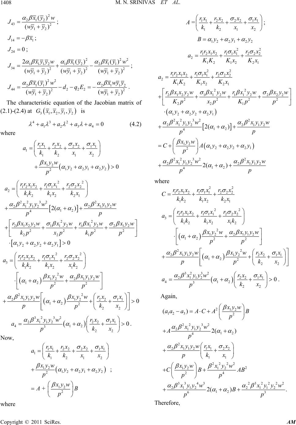
 
 

;

M. N. SRINIVAS ET AL. 1408
2
212
43 2
12
()
()
x
yw
Jwyy

;
14 1
J
x

 ;
24 0J;
22
1112 112211
34 22
12 1212
2()
()()()
2
2
()
x
yywx yx yw
Jwy ywy ywy y
 

 
;
22
2112112
4422 2
22
12 12
()
() ()
x
yw xwyy
JdqE
wy ywy y
 


.
The characteristic equation of the Jacobian matrix of
(2.1)-(2.4) at

31212
,,,Gxxyy is
43 2
1234
0aa aa    (4.2)
where

11222 211
1
12 12
12
122122
20
rx rxxx
akkx x
xywyyy
p









22
1212111222
2
12 1221
22 322
21122112
12
4
22
2122112112212
2222
221
12 22 21
2( )
0
rr x xrxrx
akkkxk x
xyyw xyyw
p
p
rxxywxywrxywxyw
kpxp kpp
yyy

 















22
121211 1222
3
12 12 12
2
122112
12 22
22
21121222 11
12 2
22
0
rr x xrxrx
akk kxxk
xy wxyyw
pp
xyywxy wrxx
pk p



 






 





 



x


32 32
211222 11
412
3
22
0
xyywrx x
akx
p
 





 .
Now,

11 222211
1
12 12
12
1221 22
2
12
2
+
rx rxxx
akkx x
xyw yyy
p
xy w
AB
p











;
11222 211
12 12
=rxrxxx Akkx x


 


;
122122
Byy y




22
121211 1222
2
12 1221
rr x xrxrx
a
K
KKxKx





22
121211 1222
2
12 1221
22
2122112112222
2222
221
12 22 21
22 322
21122112
12
4
12
12 22 21
2
22 32
2112
2( )
rr x xrxrx
aKKKxK x
rxxywx ywrx ywxyw
KpxpKpp
yyy
xyyw xyyw
p p
xyw
C Ayyy
p
xyyw
p



 














 



2
2112
12
42( )xy yw
p



where
22
12 12111222
1212 21
rr x xrxrx
C
kk kxk x




22
12 12111222
3
12 12 12
2
122 112
12 22
22
2 112122211
12 2
22
rr x xrxrx
akk kxxk
xy wxyyw
pp
x
yywxy wrxx
pk p



 






 


x













323 2
211222 11
412
3
22
0
xyywrx x
akx
p
 






. 
Again,
212
12 32
22 32
2112
12
4
2
2112 11 22
11
22 22
2
121 2
24
3343232 222
21122 112
12
63
()
2( )
2( ).
xyw
aaaA CAB
p
xyyw
Ap
xyywrxx
pkx
xywx yw
CB AB
pp
x
yy wxyyw
B
pp

 
 

 















Therefore,
where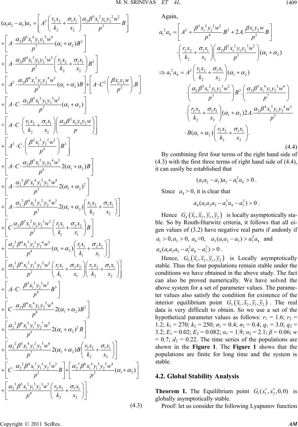

M. N. SRINIVAS ET AL.1409
32 22
2221121 12
123 33
22
54 54
2
2112
12
7
43 33
2
211222 11
5
22
43 43
22 2112 12
12
52
()
()
() .
rxxx yyw
aaa aAB
kx p
xyyw
AB
p
xyywrxx
AB
kx p
xyyw xyw
A
BAC B
pp

 
 
 










 




 
 




 
 
 
 

32 32
2112
12
3
2
22112112
22
22 22
22
12
4
3343
2112
12
6
254264
2
2112
12
7
24
2
()
+
2( )
2( )
xyyw
AC p
rx xxyyw
AC kx p
xyw
AC B
p
xyyw
AC B
p
xyyw
Ap
x
A
 


 
 



 



 
 

 







 




 



 



32 43
11 22211
12
5
22
32 22
211211 22
3
11
2432 43
21121122
12
4
11
2422 22
21 1211222211
2
11 22
2( )
()
yywrx x
kx
p
xyyw rxx
CB
kx p
xyywrx x
kx p
xyywrxxrx x
kx kx
p


 
 

 











 






 







33 33
3
12
6
44 54
2
2112
12
8
2652 75
2 2112
12
9
254254
2112 2211
12
7
22
2432 33364
2112211
5
2( )
2( )
2( )
xyw
AC B
p
xyyw
CB
p
xyyw B
p
xyywrx x
Bkx
p
xyyw xy
CB
p

 
 
 

 












 















 


354
2
12
5
3533 33
21122211
4
22
()
.
yw
p
xyywrxx
kx p

 












(4.3)
Again,
22 22
22 2
12 12
14 42
32 32
221121 12
12
3
22
22
22 11
141 2
22
32 3254 54
2
21122112
37
22 11
12
22
2.
()
()
.
(
xywxyw
aa AB AB
pp
rxxxyy w
kx p
rx x
aaA kx
xyyw xyyw
B
pp
rx x
kx



 


 


 
 


 

 












43 43
2112
5
22 11
12
22
)2 .
() .
x
yy w
Ap
rx x
Bkx




 


(4.4)
By combining first four terms of the right hand side of
(4.3) with the first three terms of right hand side of (4.4),
it can easily be established that
0
2
12331 4
()aaaaaa

.
Since > 0, it is clear that
0
4
a
22
4123 143
()aaaa aa a

.
Hence


41212
,,,Gxxyy
y Routh-Hu
is locally asymptotically sta-
ble. So brwitz criteria, it follows that all ei-
gen values of (3.2) have negative real parts if andonly if
and
0
13 4
0,0, >0,aa a 2
312 314
()aaaaaa
22
4123 14 3
()aaaa aa a

.
Hence,


31212
,,,Gxxyy
us the four populatio
ns we have obtained
be proved numeric
stem for a set of pa
es also satisfy the con
ilibrium point
is Locally asymptotically
stable. Thns remain stable under the
conditio in the above study. The fact
can also ally. We have solved the
above syrameter values. The parame-
ter valudition for existence of the
interior equ

31212
,,,Gxxyy
ain. So we use
. The real
data is very difficult to obta set of the
hypothetical parameter values as follows: r1 = 1.6; r2 =
1.2; k1 = 270; k2 = 250; σ1 = 0.4; σ2 = 0.4; q1 = 3.0; q2 =
3.2; E1 = 0.02; E2 = 0.082; α1 = 1.9; α2 = 2.1; β = 0.06; w
= 0.7; d2 = 0.22. The time series of the populations are
shown in the Figure 1. The Figure 1 shows that the
populations are finite for long time and the system is
stable.
4.2. Global Stability Analysis
Theorem I. The Equilibrium point is
globally asymptotically stable.
Proof: let us consider the following Lyapunov fun
11 2 ( ,,0,0)Gx x

ction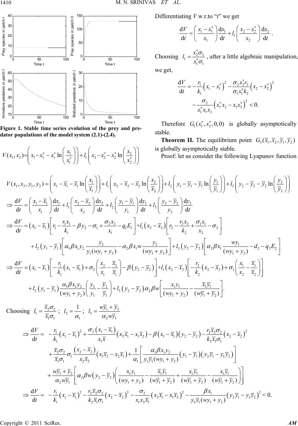

M. N. SRINIVAS ET AL. 1410
050100
0
10
20
30
40
Time t
P rey species i n pat ch I
050 100
0
50
100
150
Time t
Prey speci es i n pat ch II
050100
10
20
30
40
50
60
Time t
I m m at ure predators i n pat ch I
050 100
0
10
20
30
Time t
Mat ured predators i n pat ch I
Figure 1. Stable time series evolution of the prey and pre-
dator populations of the model system (2.1)-(2.4).
12
121 111222
12
(, )lnln
xx
x xxxxlxxx
xx
 


 


 

 

V
Differentiating V w.r.to “t” we get
11 122 2
1
12
dd
d
dd d
x
xx xxx
Vl
txt x






.
t
Choosing 22
1
11
x
lx




, after a little algebraic manipulation,
we get,
 

22
1222
112 2
111 2
2
2
12 12
112
d
d
0.
rxr V
x
xx
tk xk
xx xx
xxx










x
Therefore is globally asymptotically
11 2
( ,,0,0)Gx x

stable.
Theorem II. The equilibrium point 31 (,, ,)Gxxyy
2 1 2
is globally asymptotically stle.
Proof: let us consider the following Lyapunov function
ab
121
12121111222211132 22
121
1112 22111
12
1
2
2
(,, ,)lnlnlnln
dd d d
xxy y
Vxxyyxxxlxxxlyyyly yy
xxy y
xxxx xxyyy Vll
t








  
 
 
  




2 1
dd dtx xty
 

 
 
222
3
2
22 11
2 222
22
22 1
21 1122132221222
12 12
d
() ()()
yy y
l
tyt
r xx
x x rkx
yy wy
ly yxyxwlyyxdqE
ywyy wyywyy


 





 



 

 

11 22
11 12 1111
11
dd
d+
d
rx x VxxryqE l
tkx



  


1

112
1
d
d
Vx
t
 

 
122
1112 2
111
11222
21 1322
1211
()
rx x
xx x y
kxx
xyy y
ly ylyy
wy yyy




 
 




 



Choosing
2 11
2122 221
2 22
11 11
2
12 12
+
.
()()
r xx
ylxx xx
k xx
xy xy
wwy ywyy




 
 



 



 
22
1
11
x
lx


; 2
1
1
l

; 12
3
21
wy y
lwy



  

 
221 1
1
11 2112
11
22
22
11221
d
d
1
xx
r Vxx xxxx
tk xx
xx
x
xxxx
xxxy





 




2
222
11 222 2
211
1 12
112112
11221 1112
11 11 11
22
2112 12 12
()
()
()()
rx
xxyyx x
kx
xy
yyyyyy
ywyy
x yx yx y
wy ywyywy ywy y


 
 







1 2
2
wyy
wy




   
11
12
2 22
2 1
2 2211221 12
11 1211112
()
< 0.
()
xy
wyy
x
x xxxxxyyyy
kx xxxyywyy
 







 




2
122 2
11
12
d
d
rrx Vxx
tk
 

M. N. SRINIVAS ET AL.1411
Therefore 31 2 1 2 (,,,)Gxxyy is globally asymptoti-
cally stable.
5. Qualitative Bionomic Phenomena
dy of the
odels. Let
r prey species, be the fishing cost per unit
effort for matured predpecies, be the price per
unit biomass of the prbe thce per unit bio-
mass of the predator (m). Thnet revenue or
conomic rent at any tiby where
re-
Net
The bionomic equilibrium
It is the stu dynamics of living resources using
economic mbe the fishing cost per unit
effort fo
1
c
2
c
ator s
ey,
ature
me
Rp
dator
22
1
p
e pri
erefore
2
()c
2
R
2
p
d
given e12 RR R
2
E; here
represents
11111
()RpqxcE,
presents Net Revenue for
revenue for mature
122
qy
the prey;
d prespecies.
1
R


1212 12
() ,() ,() ,(),,xx yyE E


 is given by the
following equations
2
11
111 2112 2111
1
0
rx
rx xyxxqEx
k
   (5.1)
2
22
2211 22
2
0
rx
rxx x
k
   (5.2)
2
112 2112
12 12
0
xy xyyw
wy ywy y
 


(5.3)
2112
222 22
12
0
xyywdy qEy
wyy

 
 (5.4)
 (5.5)
In order to determine the bionomic equilibrium we
come across the following cases.
Case I. If for the matured predator, fishing cost is
greater than the revenue 2 ), then fishing of
matured predator is not fea fishing of prey
population remains operation1 ).
Thus, when an1

2
RE y.
 
1111 12222 0pqxcpqcE 
(222 cpqy
sible. Hence
al (11 cp
d cpq
1
qx
x
20E111

we have

1
1
11
c
xpq
,

22
22222
2
11
4
() 2
krc
xrr
rp








.
1
,
112
qk


Since 1 c11111 pqxpqk





21
,yE

will be
any point on the line

1
12111
111
2112211
22 22
21 112
1
4.
2
yqErpqk
pqkr c
rr
rc pqk











c

Case II. If 1 i.e., the cost is greater than the
revenue in th, then the prey fishing will be
closed (i.e. ly matured predator fiing re-
mains op2
111
cpqx
e prey fishing
1
E= 0). On
al (i.e.
sh
eration 222 cpqy

)

2
2
22
pq
Substitu
c
y.
te this value in (5.1), we get




21
211
1
( )()
cx
xx
pq




1
11
() 1x rx


222 1
k





 






.
Here


1
x

is the positive solution of
32
11213140axaxaxa

 (5.6)
where
2
12
122
122
0
rr
akk


;
12 2
211
2
22 12 2
2rr c
ar
pq
kk









;

2
221
311 2
2
221 2 22
rcr
ar r
pq k k

2


 



 ;

2
42211
22
1c
arrpq

1
2








.
2
11
22
c
rpq








 < 0 (or) 2
11
22
c
rpq






Now if > 0,
then
2
2212
11
2
2212 22
()rcrr
rpq k
k
2






 


2
22111
22
() c rrpq

2






. and 
Then Equation (5.6) has a unique positive solution


11
x
x




2
x

to be positive, we must have For

21 11
11
2211
ck k
xk
pqr r

 .
Substitute the value of

1
x
 in Equation (5.4), we
get


 
 
21 1
2
1xyw
E
qwy y


2
212
d













20,E Provided

121
xd  

2
2
where
1
 



12
21
y

y
w



.

M. N. SRINIVAS ET AL. 1412
Case III. If 2 , then the co
greater than re and the
fishery will be closed.
Case IV. If 2 , th
nues for both th
fishery will be in operation.
In this case
111
cpqx,
venues for
1222
cpqy
both the species
st is
whole
111
cpqx,
he species b
1222
cpqy
eing positive, t
en the reve-
en the whole

1
1
11
c
xpq
 (5.7)

2
2
22
c
ypq
. (5.8)
Substitute (4.7) and (4.8) in (4.1), (4.2), (4.4) we get

2
k

211
22222
2
4rc
112
() 2 xrr
r


pqk





(5.9)

11 21221
1
11
()
1
rc cxp
Eqpqkqpq c




 

 (5.10) 1 1 2 11
q
 1 2 1
q


211
22
212
() 1xyw
Ed
qwyy








(5.11)
if

10E
1122121
11111221
()
1
rc xpc
pqkqcqpqq
1 1
q




 
 (5.12)
if



20E
121
2
1211
cd
pq
 


. (5.13)
The Non-trivial Bionomic equilibrium point


12 212
() ,() ,() ,() ,xx yEE


exists if (5.12d
(5.13) hold.
in this section we employ the
Pontryagin’s maximum principle tbtain a path of op-
timal harvesting policy so that if the fish populations
inre kept along this
path, then the regulatory agency is assured to achieve its
objective. We consider the following present value J of
continuous time-stream
) an
6. Optimal Harvesting Policy
In this section we study optimal harvesting policy of the
system (2.1)-(2.4). Also
o o
side and outside the reserve zones, a
a

1212 1 2
,,,,,,e
0
d
t
J
Px xyyE Et
t


 (6.1)
where is the net revenue given by

(6.2)
and
P


1212 1 2
11111222 22 2
,,,,,,PxxyyEE t
pqxEcEp qy Ec E 
1
denotes the instantaneous annual rate of dis-
count, the aim of this section is to maximize
J
sub-
jected to the state Equations (2.1).
Firstly we construct the following Hamiltonian func-
tion

)-(2.4




111112 2222
1
E
y
1
1111 2 11 211
1
2
2 1
2
21
3112212
12 12
1
421222 22
12
ee
1
1
tt
HpqxcE pqyc
x
rxx yxxqEx
k
x
k
yw
xy xy
wyywy
wy
xydyqy
wyy



 


 

2
22122
rxxx  
2
E
y


 

 



















w
 



(6.3)


here 1234 ,,,

 are additional unknown functions
are the control vari- called the adjoint variables, 12
,EE
ables satisfying the constraints

11
max
0EE;


22
max
0EE , and


11111
()e t tpqxc



,
111
qx


222 22
()e t tpqyc
 
 are called the switch-
ing f
2 42
 qy 
unctions.
We aim to find an optimal equilibrium









 


1212 1 2
,,,,,xxyy EE

  
Hamiltonian
to mize maxi
H
.
Since Hamiltonian
H
al
ontro
is linear in the control vari-
ables control can xtreme con-
trols gular cls, thus we have
ax
1
,EE
or the sin
2
, the optimbe e
1
(EE
1m
)

() 0t, when 1


i.e., when 1
11
11
etc

 ; ()tp
qx

10E

, when 1() 0t


i.e., when 1
11
11
etp

 ; () c tqx 
22max
()EE

, when 2()t0


i.e., when 2
42
22
()etc tp
qy

  ;
20E

, when 2() 0t


2
42
22
()etc
tp
qy

 
i.e., when ;
when ()0t
1


, 1 ()etc tp

  ;
11
11
qx
or
1
0
H
E


 6.4) (

M. N. SRINIVAS ET AL.1413
when 2() 0t

, 2
42
22
()etc
tp
qy

  ;
or
2
0
H
E


.
In this case, the optimal control is called the singular
control, and (6.4), (6.5) are the necessary conditions for
the maximization of Hamiltonian
(6.5)
H
.
By Pontrayagin’s maximal principle, the adjoi
tions are
nt equa-
1
1
δt11
11 1112111
σyqE
1
2
212
4
12
d
d
2 r x
epqE λr
()
H
tx
k
ywyy wyy
wyy
122 12
21 3
12 12
λσ
wy ywyy







 










  










(6.6)
222
122 22
22
d2
d
rx
Hr
tx k
 



 
 



(6.7)
3
1
2
112212 2
3
12
d
d
(
H
ty
22
12
21 22
42
)()
()
12
x
yw xywy
wy

 




 



(6.8)
ywy y
xywy
wy y












4
2
1 1
22
211
4222
2
12
d
.
()
t
ty
22 21 1
222
11 1222
e()
2
pqE x
xyywy
322
12 12
() ()
dH
x
wy
 







(6.9)
wy ywyy



xw ydq
E
wyy








 



 



Considering the interior equilibrium




31212
,,,Gxxyy
as

and Equations (6.4), (6.7), can be written
2
212
d() e
d
t
AA
t




where 22 11
1
22
rx x
Akx

; 1
21
11
c
Ap
qx 2





.
We can calculate that
2
2
1
et
A
A



. (6.10)
larly, by conSimisidering the interior equilibrium


31212
,,,Gxxyy and Equati.5), (6.8), can be wri- ons (6
tten as 3
det
3 4
d3
A
A




t
where
212
3
12
;
wx y
Awyy



2
2212
42 2
cwxy
Ap
qy wy y





22 12






clu that
.
We can conde
4
3
3
et
A
A



. (6.11)
interior equilibriumSimilarly, by considering the


,y and
312
,,Gxxy Equations (6.10), (6.11), (6.6) can
as
12
be written 1
15 6
de
d
t
A
A
 
t


where
1
5
rx
Akx 
122
11
x 
;

24
AA
611 1 11221
13
2212
221 2
.
A
2
pqEy wy
AA
cwyy
qyy y



 

 
 

 
conclude that
pw 



We can
6
1
5
et
A
A



. (6.12)
Similarly by considering the interior equilibrium


3
G12 ,,,xxyy and Equations (6.10), (6.11), (6.6) can
be written as
12
4
47
d
d8
et
A
A
 
t


where

2
y2
21 1
7222
2
12
xw dqE
wyy


;
A
64212
.
822 2 1
A
5312
A
xwy 


Apq E x
AAwyy


 
 

We can calculate that
8
4e
At
7
A




 
It is obvi
. (6.13)
ously that 1234 (), (), (), ()tttt

 are bound-
ed as
Substitute (6.12) in (6.4), we obtain a singular path
t.
6 1
1
11 5
A
c
pqx A


. (6.14)
Substitute (6.13) in (6.5), we obtain a singular path

M. N. SRINIVAS ET AL. 1414
8 2
2
22 7
A c
pqy A


. (6.15)
Using

2
221
22222
22
4
2
krx
xr r
rk







1





2
11
2111112
11
1rx
yrqEx
xk






,
2
x 
12345678
,,,,,,,
A
AAAAAAA can be written as

1
2
2211
122 22
2
211
1/2
2211
22 22 2
2
4
11
()
22
2
4
()()
rx
Arr k
rx
rx
kr rk






 



 



1
21
11
c
Ap
qx 2





12 11
31
12 11
wxc
Ap
qx
 
2







2
42 2
21
11111 22
11
c
Ap qrx
rqEx x
xk


 



1

1/2
2 112 2211
52222
112 2
4
()()
2
rxkrx
Arr
kxr k




  





1
12
11
6111
22 11
pqx
Ap
q Erx x






22
1 1
22
12
11
1 11 22
1
)
c
kx
cx w y
rx
Ex x
k


















 



2
2 2
+p




22 2
(qr q 





2

2
121
x
7222
2
12
A
dqE


 
2
A6421
2 2 1
5312
+
82
A
xw 

Ap xq EAA 
 
 


.
(6.14) and (6.15) can be written as Thus

6 1
11
11 5
A
c
Fxp qx A


 



and


8 2
22
22 7
A
c
Gyp qy A


 



.
There exists a unique po11 ()
x
x

 of sitive root


10Fx

in the interval 11 0
x
k If the following
hold F (0) <0, F) > 0, (1
k

10x for F
10x, and
22
()yy


Similarly There exists a unique positive root
of


20Gy

in the interval 22 0yk If the
) < 0, G (2 k) > 0,
fol-
lowing hold G (0

20Gy
 for
20y.
For 11 ()
x
x


, 22 ()yy


,
we get

2
22
22222
2
4
() 2
kr
xr r
rk



11
x









21
2
1
()
() wy y




;

2
11
1
11111122
1
()
() ()
rx
yrqEx x
k

21
xw











1
11
1
1112112 2
() ()()()( ) xxyxx

1
1
() ()
() 1
Eqx
rx k




 





 

 





21 12
2
()Ed
22
221 2
()()( ()
()() ()
xyyw y
qywy y
 
)
1












i.e., 21 1
22
212
()( )
1
() ()( )
xyw
Ed
qwyy











.
Hence once the optimal equilibrium,


1212
(),( ),(),( )xx yy

 
is determined, the optimal
harvesting effort 1 ()E

and 2 ()E

(6.11), (
can be determined.
From (6.3), (610),
found that
.4), (6.6.12) and (6.13), we
()
it

where = 1, 2, 3
timri. Hence they rem
7.
We have considered a system of tw
fe ui-
lib is
stable. We have shown the stability r
and also numerically. We can also considered a delayed
mm to take into account of the gestational de-
lay of the matured predator population. It is natural that
the consumption on the prey by the predator needsome
time to contribute to the biomass of the predator. So we
use delay differential Equation (7.1) to study sue-
nomena.
i
um
, 4, do not vary with
e in optimal equilibain bounded
as t .
Computer Simulation Discussion
o populations at dif-
rent stage structure. The stability of the interior eq
rium point is studied and it is shown that the system
esults analytically
odel syste
s
ch ph
2
111
111 2112 21
yxxq   
11
1
d
d
xrx
rx xEx
tk
  

M. N. SRINIVAS ET AL.1415
2
222
221122
2
d
d
xrx
rxx x
tk
  (7.1)
2
11 122 112
12 12
d
d
yxy xyy
twyy wyy
 


w

21 12
2
222 22
12
d
d
xt yyw
ydy qEy
twyy
  

.

Delay differential equation models are studied exten-
sively in the study of several ecological systems by K.
Das and N. H. Gazi [26,27]. All those systems are two
and three dimensional systems. Since the present model
is four dimensional system, the analytical study of the
system is difficult to tractable and the expression for the
delay parameter values will be complicated for which the
system is stable. So, we solve the system numerically
only. The numerical solutions are shown in the Figures
2-5. The Figures 2 and 3 show the stable solution of
510 15 20 25 30 35 40
29
30
31
32
33
34
35
36
37
x 1- unreserved prey
x 2- res erved prey
Figure 2. The stable phase portrait of prey in unreserved
zone verses prey in reserved zone for delayed model stem
(7.1).
sy
050 100
0
10
20
30
40
time
s pecies in patchPrey I
050100
0
50
100
150
time
Prey species in patch II
050 100
0
50
100
150
tim
I m patch I
e
mature predat ors in
050100
0
50
100
150
time
. The stable time series evolution of the prey and
populations of the delay model system (7.1) for τ <
10.
Matured predat ors in patch I
Figure 3
predator
050 100
0
10
20
30
40
time
Prey speci es in patch I
050 100
0
50
100
150
time
Prey speci es in patch II
050 100
0
0.5
1
1.5
2x 10
7
time
I m m ature predat ors i n patch I
050 100
0
0. 5
1
1. 5
2x 10
7
time
Matured predat ors i n patch I
Figure 4. The unstable time series evolution of the pr and
predator populations of the delay model system (7.1).
ey
00.2 0.40.6 0.8 11.2 1.41.6 1.8 2
x 10
7
0
2
4
6
8
10
12 x 10
6
Immat ure predators in pat ch I
Figure 5. Unstable phase-portrait of the predator popula-
tions for the delayed model system (7.1) with delay pa-
rameter value τ ≥ 10.
the populations for τ ≤ 10 while the Figures 4 and 5
show that the system is unstable for τ > 10.
8. Ackn
Mat ured predat ors in
owledgements
Authors are thankful to the reviewers for their vaable
constructive comments and suggestions to improve this
paper.
9. References
[1] F. Brauer and A. C. Soudack, “Stability Regions and
Transition Phenomena for Harvested Predator-Prey Sys-
tems,” Journal of Mathematical Biology, Vol. 4,
patch I
lu
7, No.
1979, pp. 319-337. doi:10.1007/BF00275152
F. Brauer and A. C. Soudack, “Stability Regions in Pre-[2]

M. N. SRINIVAS ET AL. 1416
dator-Prey Systems with Constant-Rate Prey Harvesting,”
Journal of Mathematical Biology, Vol. 8, No. 1, 1979, pp.
55-71. doi:10.1007/BF00280586
[3] G. Dai and M. Tang, “Coexistence Region and Global
Dynamics of a Harvested Predator-Prey System,” SIAM:
SIAM Journal on Applied Mathematics, Vol. 58, No. 1,
1998, pp.193-210. doi:10.1137/S0036139994275799
[4] M. R. Myerscough, B. E. Gray, W. L. Hograth and J.
Norbury, “An Analysis of an Ordinary Differential Equa-
tion Model for a Two-Species Predator-Prey System with
Harvesting and Stocking,” Journal of Mathematical Bi-
ology, Vol. 30, 1992, pp. 389-401.
[5] K. S. Chaudhuri and S. S. Ray, “On the Combined Har-
vesting of a Prey-Predator System,” Journal of Biological
Systems, Vol. 4, No. 3, 1996, pp. 373-389.
doi:10.1142/S0218339096000259
[6] A. W. Leung, “Optimal Harvesting Co-Efficient Control
of Steady State Prey-Predator Diffusive Volterra-Lotka
Systems,” Applied Mathematics & Optimization, Vol. 31,
No. 2, 1995, pp 219-241. doi:10.1007/BF01182789
[7] C. W. Clark, “Mathemalical Bioeconomics: The Optimal
Management of Renewable Resources,” John Wiley and
Sons, New York, 1979.
[8] S. A. Levin, T. G. Hallam and J. L. Gross, “Applied
Mathematical Ecology,” Springer-Verlag, Berlin, 1989
/0025-5564(90)90019-U
.
[9] W. G. Aiello and H. I. Freedman, “A Time Delay Model
of Single Species Growth with Stage Structure,” Mathe-
matical Biosciences, Vol. 101, No. 2, 1990, pp. 139-153.
doi:10.1016
H. I. Freedman and K. Gopalsammy, “Global Stability in
Time-Delayed Single Species Dynamics,” Bulletin of
Mathematical Biology, Vol. 48, No. 5-6, 1986, pp. 485-
492.
[11] G. Rosen, “Time Delays Produced by Essential Nonlin-
earity in Population Growth Models,” Bulletin of Mathe-
matical Biology, Vol. 49, No. 2, 1987, pp. 253-255.
[12] M. E. Fisher and B. S. Goh, “Stability Results for De-
layed Recruitment Models in Population Dynamics,”
Journal of Mathematical Biology, Vol. 19, No. 1, 1984,
pp. 147-156. doi:10.1007/BF00275937
[10]
[13] M. Mesterton-Gibbons, “On the Optimal Policy for the
Combined Harvesting of Predator and Prey,” Natural
Resource Modeling, Vol. 3, 1988, pp. 63-90.
[14] C. W. Clark, “Mathematical Bioeconomics: The Optimal
Management of Renewable Resources,” Wiley, New
of a Multi Species Fishery,” Ecological Modelling, Vol.
32, No. 4, 1986, pp. 267-279.
doi:10.1016/0304-3800(86)90091-8
York, 1976.
[15] K. S. Chaudhuri, “A Bio Economic Model of Harvesting
[16] D. L. Ragozin and G. Brown, “Harvest Policies and Non
Market Valuation in a Predator Prey System,” Journal of
Environmental Economics and Management, Vol. 12, No.
2, 1985, pp. 155-168. doi:10.1016/0095-0696(85)90025-7
[17] A. Hastings, “Global Stability of Two Species Systems,”
Journal of Mathematical Biology, Vol. 5, 1978, pp.399-
403.
[18] X.-Z. He, “Stability and Delays in a Predator-Prey Sys-
tem,” Journal of Mathematical Analysis and Applications,
Vol. 198, No. 2, 1996, pp. 355-370.
doi:10.1006/jmaa.1996.0087
[19] B. S. Goh, “Global Stability in Two Species Interac-
tions,” Journal of Mathematical Biology, Vol. 3, No. 3-4,
1976, pp. 313-318. doi:10.1007/BF00275063
[20] W. G. Aiello and H. I. Freedman, “A Time Delay Mode
doi:10.1016/0025-5564(90)90019-U
l
of Single Species Growth with Stage Structure,” Mathe-
matical Biosciences, Vol. 101, No. 2, pp. 139-153.
[21] W. G. Aiello, H. I. Freedman and J. Wu, “Analysis of a
Model Representing Stage Structured Population Growth
with State-Dependent Time Delay,” SIAM: SIAM Journal
on Applied Mathematics, Vol. 52, No. 3, 1992, pp. 855-
869.
[22] T. K. Kar and M. Swarnakamal, “Influence of Prey Re-
serve in a Prey-Predator Fishery,” Non-Linear Analysis,
Vol. 65, No. 9, 2006, pp.1725-1735.
[23] W. Wang and L. Chen, “Optimal Harvesting Policy for
Single Population with Periodic Coefficients,” Mathe-
matical Biosciences, Vol. 152, No. 2, 1998, pp. 165-177.
doi:10.1016/S0025-5564(98)10024-X
[24] R. Zhang, J. F. Sun and H. X. Yang, “Analysis of a Prey-
Predator Fishery Model with Prey Reserve,” Applied Ma-
thematical Sciences, Vol. 50, No. 1, 2007, pp. 2481-
2492.
[25] W. D. Wang, Y. Takeeuchi,Y. Saito and S. Nakaoka,
“Prey-Predator System with Parental Care for Predators,”
Journal of Theoritical Biology, Vol. 241, No. 3, 2005, pp.
451-458. doi:10.1016/j.jtbi.2005.12.008
[26] K. Das, N. H. Gazi, “Structural Stability Analysis of an
010, pp. 2191-
ontrol of Parameters of a De-
Algal Bloom Mathematical Model in Trophic Interac-
tion,” International Journal of Non-linear Ananlysis:
Real World Applications, Vol. 11, No. 4, 2
2206.
27] N. H. Gazi and K. Das, “C[
layed-Diffusive Autotroph-Herbivore System,” Interna-
tional Journal of Biological System, Vol. 18, No. 2, 2010,
pp. 509-529.