Applied Mathematics, 2011, 2, 1382-1386
doi:10.4236/am.2011.211195 Published Online November 2011 (http://www.SciRP.org/journal/am)
Distribution of Geometrically Weighted Sum of Bernoulli
Random Variables
Deepesh Bhati1, Phazamile Kgosi2, Ranganath Narayanacharya Rattihalli1
1Department of Stat i s t i c s, Central University of Rajasthan, Kishangarh, India
2Department of Stat i s t i c s, University of Botswana, Gaborone, Botswana
Received July 6, 2011; revised October 5, 2011; accepted October 13, 2011
Abstract
A new class of distributions over (0,1) is obtained by considering geometrically weighted sum of independ-
ent identically distributed (i.i.d.) Bernoulli random variables. An expression for the distribution function (d.f.)
is derived and some properties are established. This class of distributions includes U(0,1) distribution.
Keywords: Binary Representation, Probability Mass Function, Distribution Function, Characteristic Function
1. Introduction
Uniform distribution plays an important role in Statistics.
The existence of uniform random variable (r.v.) over the
interval (0,1), using B(1,1/2) r.v.s is indicated in [1]. As a
generalization, in this paper we consider the following
geometrically weighted sum of i.i.d. Bernoulli r.v.s
1
1
2
j
j
j
X
Z





, (1)
where
j
Z
s
 are i.i.d. B(1,p) r.v’s. The remainder of the
paper is organized as follows. In Section 2 we obtain the
characteristic function of X and give an interpretation for
the variable X. In Section 3 we derive the distribution
function of X and prove some of its properties. In Section
4 we discuss the existence of the density function. In
Section 5 distribution of sum of a finite number of vari-
ables is considered and the graphs of its probability mass
function (p.m.f.) and distribution function (d.f.) are given
in the Appendix.
2. The Characteristic Function and an
Application of the Model
2.1. The Characteristic Function
Let

()

F
tPXt
be the d.f. of X. Then by the defi-
nition of X we have





11 11
()001 1
1
(1 ).
222
FtP XtZPZPXtZPZ
XX
PtpP tp
 
 

 
 
(2)
Hence the characteristic function (c.f.) ()t

of X
satisfies the equation
2
()(1)( 2)e(2)
it
tptpt  .
That is,
2
()(2) 1e
it
tt pp

 

.
Repeating this and replacing t by 2t each time, we
get, for n = 1, 2,.
2
1
()(2 )1e.




k
n
nit
k
tt pp (3)
The reproductive property of the characteristic func-
tion exhibited by (3) is comparable to the characteristic
function of an infinitely divisible distribution. For details
one may refer to Section 7 of [2].
Since (2)1 as
n
tn

 we have
2
1
()1e k
it
k
tpp




 


. (4)
Note that if p = 0, this infinite product is 1, and, if p =
1, the infinite product is . Thus p = 0 results in X be-
ing degenerate at 0 while p = 1 implies that X is degene-
rate at 1. If p = 1/2, then the product term in (4) is
eit
2
1e 1e 1
2e1
n
it it
nit it



 as n

Thus if p = 1/2 then X has U(0,1) distribution.
2.2. An Application
This resulting distribution can be used as a model in a

D. BHATI ET AL.1383
1
,
situation similar to the following. Suppose a particle has
linear movement on the interval [0,1]. To capture the
particle suppose the following binary capturing tech-
nique of dividing the existing interval into two equal
halves is used. Suppose initially there are two barriers
put at 0 and 1. After one unit of time a barrier is put at
the midpoint of 0 and 1. Further the interval in which the
particle is found is divided into two equal halves by
placing a barrier at their midpoint and the process is con-
tinued. The intervals containing the particle keep on
shrinking and finally shrink to X, the point at which the
particle is captured in the long run. The behavior of the
particle is known only to the extent that at the moment of
placing a barrier after exactly one unit of time the parti-
cle is on the right side of the inserted barrier with prob-
ability p.
3. Main Results
3.1. Notation
It is known that every number t, has a binary
representation through as
0t
,0or1

1
nn
aa

1
1
2
i
i
i
ta





. If a number t has the representation
1
1, 1,
2
i
k
ik
i
ta a







we refer t as a finite binary termi-
nating number and such a number can be represented by
for some . However such a
number also can be represented as
2,
k
r1, 2,,21
k
r
1
1,,1,2,,
2
0,1,1, 2,
i
iii
i
ki
bbai k
bbikk


  





1,
It is to be noted that the right tail of the sequence {ai}
is of the form (0,0,0 while that of the sequence {bi} is
of the form (1,1,1, In the following as a matter of
convention we do not consider representation with the
right tail of the form (1,1,1,). Under such a convention,
corresponds to a unique binary sequence
)
).
[0,1]t

1
i
a and conversely. If
1
1
2
i
i
i
ta





, then we shall
denote this relation as , (BR to mean the binary
representation).

BR
n
ta
3.2. Properties
Theorem 1:
Let and

BR
n
ta
1
k
kj
j
s
a

, . Then
the d.f. of X defined in (1) is given by
0
1, 2,,0ks


11
1
() jj
js s
j
j
FtP Xtaqp




 
. (5)
Proof:
Let,
1
1
2
i
i
i
ta





 and r be the rth non-zero element
k
a
in the sequence


,1,2,
i
ar. Let be the number
having the binary representation 12 r
k
and 0
r
t
,aa(,, 0,0,)a
0t

. It is to be noted that r is a finite binary
terminating number. If t is not a finite binary terminating
number then the sequence increases to t. If t is a
finite binary terminating number then we note that r
t
tt

r
t

for some finite r. For example, let have a binary rep-
resentation 00010011000 and
t
1234
4,7, 8, 11kkkk

 so that 1
B
R
t (001000,
2
0)
B
R
t

(00011003 00 0),
B
R
t (000100110
so on. We note that 1
i
a
00 ) and

for ,,ik k and 0
12 3
,k
otherwise. Note that


PXt


,1, 2,,1,1,0,1, 2,...
1,0,1, 2,0.


  
  


rr
rr
r
iir kkj
kkj
PZ aik ZZj
PZ Zj
Thus F does not have a jump at tr and




r
F
tFt.
ng number. WLet t be not a finite binary representie
note that



1
1
11
00,,
k
k
XtPZ Zq P0



111
2
2
121 11
1
0, ,0,1,0,
,0
kkk
k
k
PtX tPZZZZ
Zqp



 






111
3
222 3
23 111
22
11
0, ,0,1,0,
,0,1,0,,0
kkk
k
kkk k
PtX tPZZZZ
.
Z
ZZZ qp



 
 


Thus in general for r = 1, 2, 3, we have 


(1)1 rr  
1.
r
k
rr
PtX tqp
 
Hence
.

(1)1
1
11
() r
kr r
rr
rr
PX tPtXtqp





 

,
r
kj

If we let then s, then we
will have
In fact F does not have jump at ant t, (0 < t < 1).
Hence
1
1
1
1
j
ij
i
ra


 


11
.
jj
js s
q p



1
j
j
a



()PX t


11
1
.
jj
js s
j
j
PX tPXtaqp


 



D. BHATI ET AL. 1384
t is a finite binary termination number
th for some finite number r and
since
articular Case
However, if
en ttr

r
rjs s
tPXtPX t


 


11 11
11
jj jj
js s
rj j
jj
PX
PXta qpaqp
 



 

Theorem 4:
For
0,1, 2,
j
ajrr.
3.3. P
If 1
p, then

2

1
1,(0,1)
2
j
j
j
PXt att



 


.
ct it can befied that (5) satisfies (2). It fol-
fact that if t has binary representation a =
(a
Hence ~(0
Remks: ,1)XU . ar
In Fa veri
lows from the
1, a2,) then for
1) 0 < t < 1, t/2 has binary representation 12
(, ,
)
uuu
where u= 0 and ui+1 = a,i = 1, 2, and
1i
tation
1 2an, 0,
2n rpectithen
t
Theorem 3:
with
2) 1/2 < t < 1, 21t has binary represen
rv =

12
,,vv whee vi = ai+1, i = 1, 2,.
Theorem 2:
If u and vhave binary representations (a, a,,
0, , a,,a, 1, 1,,1) es,0) and (a1vely
he
2
conditional distribution of X given u ≤ X ≤ v is that of

n uX.
Proof: Follows by the definition of X.
R
Let

B
ta with

12
,,,,0,0,
k
aa a
n1 k
a

.
Then for 1 0s2k 

1
0 P

 

002
2
k
k
XtsXt PXs

  


.
Proof:




1
02
ts

 we have

11
22
q
PtXs PtXs
p

 


.
Proof:
Let




(2)
1123
,,,ZZZZZZ  ,






(2)
1
(2) (2)
1
0,
0
Pt XsPZZA
PZPZ AqPZ A
 
 
and

(2)
1
11 1,
22
PtX sPZZA

 






(2) (2)
11.PZ ApPZ A

In the above in fact
PZ 

(2) .
2
X
PZAPst

 


Hence the result.
5: Theorem
(.,If )
F
p and are the diribution functions
of respen
If
(., )Gp
ectively th
st
X an) d 1-X
Proof:
(,(,1)Gxp Fxp.
1
1
2
j
j
j
X
Z





 and
j
Z
’s are i.i.d. ),1( pB then

11
11
11
22
jj



1122
1
1122
1122
0
1122
002
0
002
02
1
,,,,
2
,,,
11
,,, 22
,,,
k
k
k
j
kk j
jk
kk
kj
kk j
j
PXtsXt
PXts
PXtstt PXt
PZ aZaZaZs
PZ aZaZa
PZa ZaZaPZs
PZ aZa







 





 





 


 
 

 
 
















12.
2
kk
k
k
Za
PXsPXs








j
j
jj
ZY

 
 
 
 

X

 where Yj’s are i.i.d.
(1,1 )Bp

.
Hence the result.
Mean and Va ri an ce of X:

1j1
1
() 22
jj
jj
EXEZpp


 
1


 





2
2
11
21
2
11
1
2
1
2
() 2
11
1
2
22
11
21
322
1(1
2











 


 
 

 
 



 


 

jij
1
1
11
2( )
2
 

 

 


i
1
2



33




j
ij
j
E EZZ
i
j
jij
i
ji
ii
i
X EZ
pp
pp
pp
p
j
2)
3
p
Hence (1 ) () .
pp
Var X 
3
By using the c.f. 2
1
()1e k
it
k
tpp



 

 the cu-
mulants can also be obtained.

D. BHATI ET AL. 1385
4. Nonexistence of Density Function
We have proved that the distribution function of X is
given by Let the
left derivative and the right derivative of F at t exist.
These be denoted by

11
1
() jj
js s
j
j
Fta qp



,

BR
n
ta.
()
f
t and ()
f
t respectively
Consider
.
1
2
f 


and 1
2
f



, the right and left de-
rivatives of F at 1/2.
1
1
111
122
2
lim
2
lim2
k
k
k





2
lim(2 )(2)
k
k
kk
FF
f
qp qp


 
 
 



k 
and

1
1
limlim(2)(2 ).
2
k
k
kk
pq pq


 

11 1
22k
k
k






at
122
2
lim
k
FF
f



 

Note th1
2
f  a


nd 1
2
f 

are equal if and
only if


1
pq. He
2t differentiable at 1/2 if nce F is no
1
2
p.
Let :1,2,3,0,1,2,,2
2
k
k
r
Dk r






. It can be
that F is not differentiable at each point of D and
D is countable dense subset of [0,1]. Hence F is
nowhere differentiable in [0,1].
5. Distribution of Sum of a Finite Numbr of
Bernoulli Random Variables
Since F(t) is an infinite series for t not in D, the exact eva-
lu is not pe for eac
ing we se-
over, the density function of X does not exist on the in-
terval (0,1). Hence in the follow consider the
quence {Xk} of r.v. defined by
shown
the set
e
ation of F(t)ossiblh (0,1).t More-
1
1.
2
i
k
ki
i
X
Z




 (6)
The sequence


k
X
increases point wise to X and
2.
k
k
XX


Similar to (5), it can be shown that for
1
1
2
j
j
j
ta





,
k

11
1
()( )
jj
js s
kj
j
F
taqpF





the d.f. of Xk is s,
wh
j
ere
1
1.
2
k
j
sa



Further, at these values of s,
j
() ()
k


F
sFs

and
va
the difference between two successive
lues of
s
’s is 2k

, as such the two functions ()
k
F
t
and ()
F
t are almost alike. Si
iso X the
nce the sequen
sequence {Fk(t)} de
ce {Xk}
creasesincreases point we t
to F(t) for (0, 1)t

.
k
We note that for p = 1/2, ()( )
F
tFs. The gra
5
phs of
p.m.f anX10 for different values of d d.f. of X and
1
2
p

are gi
H. J. Vama
of the
paper.
. References
] S. Kunte and R. N. Rattihalli, “Uniform Random Vari-
n, Academic Press, Cambridge, 2001.
ven in the Appendix.
6. Acknowledgements
We are thankful toor Professn, Central Uni-
versity of Rajasthan, India, for the discussions which
helped to improve the content and the presentation
7
[1
able. Do They Exist in Subjective Sense?” Calcutta Sta-
tistical Association Bulletin, Vol. 42, 1992, pp. 124-128.
[2] K. L. Chung, “A Course in Probability Theory,” 3rd Edi-
tio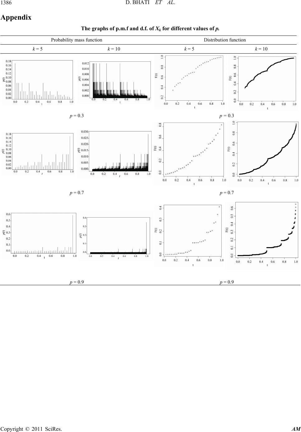

D. BHATI ET AL. 1386
Appendix
The graphs of p.m.f and d.f. of Xk for different values of p.
Probability mass function Distribution function
k = 5 k = 10 k = 5 k = 10
p = 0.3 p = 0.3
p = 0.7 p = 0.7
p = 0.9 p = 0.9