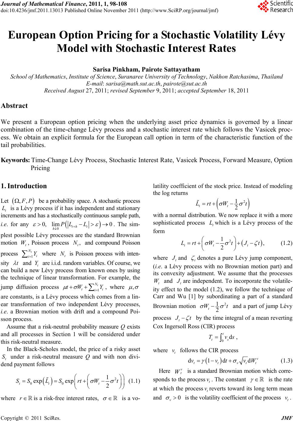
 Journal of Mathematical Finance, 2011, 1, 98-108 doi:10.4236/jmf.2011.13013 Published Online November 2011 (http://www.SciRP.org/journal/jmf) Copyright © 2011 SciRes. JMF European Option Pricing for a Stochastic Volatility Lévy Model with Stochastic Interest Rates Sarisa Pinkham, Pairote Sattayatham School of Mathematics, Institute of Science, Suranaree University of Technology, Nakhon Ratchasima, Thailand E-mail: sarisa@math.sut.ac.th, pairote@sut.ac.th Received August 27, 2011; revised September 9, 2011; accepted September 18, 2011 Abstract We present a European option pricing when the underlying asset price dynamics is governed by a linear combination of the time-change Lévy process and a stochastic interest rate which follows the Vasicek proc- ess. We obtain an explicit formula for the European call option in term of the characteristic function of the tail probabilities. Keywords: Time-Change Lévy Process, Stochastic Interest Rate, Vasicek Process, Forward Measure, Option Pricing 1. Introduction Let ,, P be a probability space. A stochastic process t is a Lévy process if it has independent and stationary increments and has a stochastically continuous sample path, L i.e. for any 0, 0 lim 0 th t hPL L . The sim- plest possible Lévy processes are the standard Brownian motion , Poisson process and compound Poisson process where is Poisson process with inten- t W N i , t N 1 t i Y t N sity t and i are i.i.d. random variables. Of course, we can build a new Lévy process from known ones by using the technique of linear transformation. For example, the Y jump diffusion process , where 1 t N t i tW Y i, are constants, is a Lévy process which comes from a lin- ear transformation of two independent Lévy processes, i.e. a Brownian motion with drift and a compound Poi- sson process. Assume that a risk-neutral probability measure Q exists and all processes in Section 1 will be considered under this risk-neutral measure. In the Black-Scholes model, the price of a risky asset t under a risk-neutral measure Q and with non divi- dend payment follows S 2 00 1 exp exp2 tt t SSL SrtWt (1.1) where is a risk-free interest rates, r is a vo- latility coefficient of the stock price. Instead of modeling the log returns 2 1 2 tt Lrt Wt with a normal distribution. We now replace it with a more sophisticated process which is a Lévy process of the form t L 2 1, 2 tt t LrtWt J t (1.2) where t and t denotes a pure Lévy jump component, (i.e. a Lévy process with no Brownian motion part) and its convexity adjustment. We assume that the processes and t Wt are independent. To incorporate the volatile- ity effect to the model (1.2), we follow the technique of Carr and Wu [1] by subordinating a part of a standard Brownian motion 2 1 2 t Wt and a part of jump Lévy process t t by the time integral of a mean reverting Cox Ingersoll Ross (CIR) process 0d t ts Tvs , where follows the CIR process t v d1d d v ttvt vvtv t W (1.3) Here is a standard Brownian motion which corre- sponds to the process. The constant v t W t v is the rate at which the processreverts toward its long term mean and t v 0 v is the volatility coefficient of the process . t v 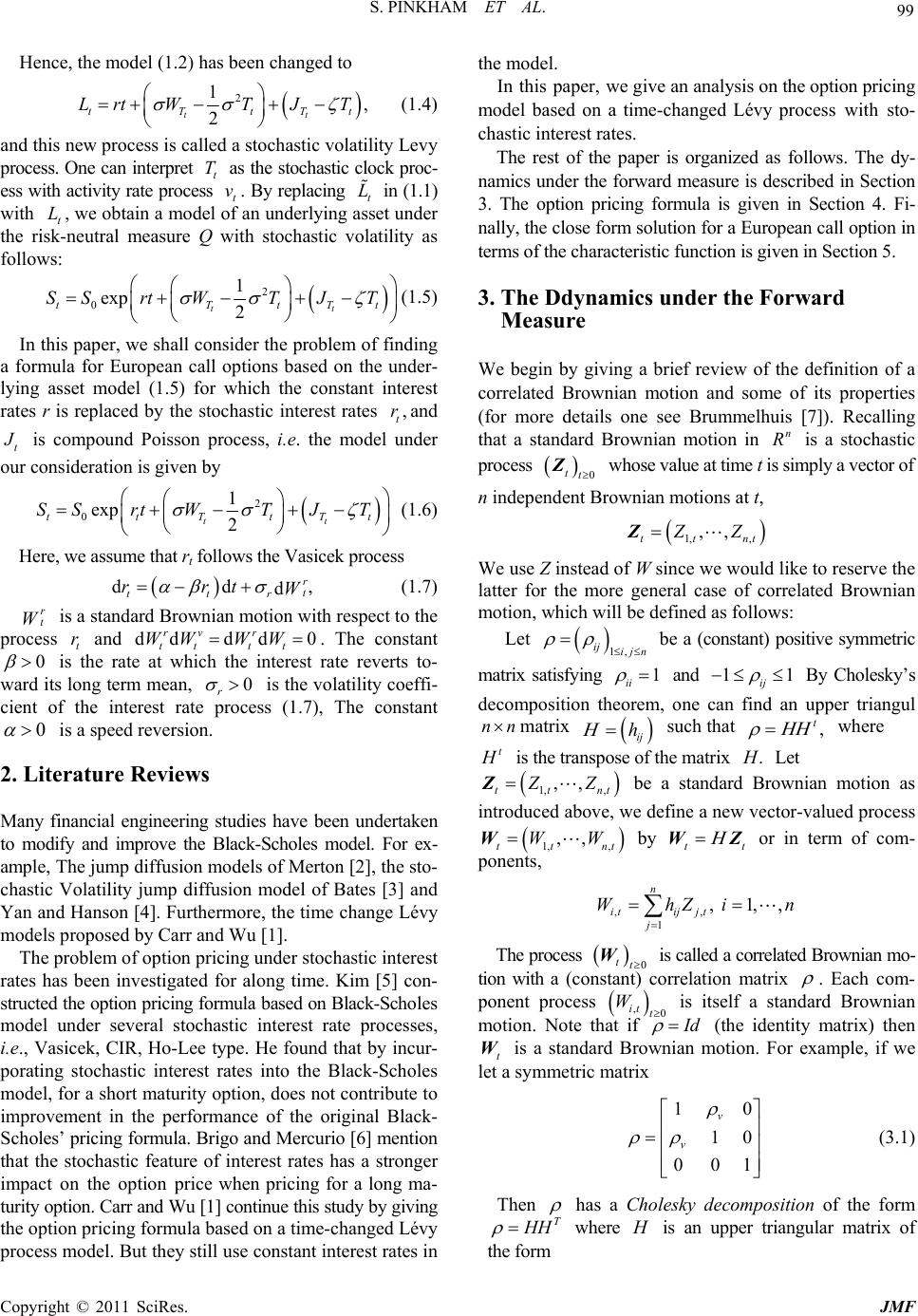 99 S. PINKHAM ET AL. Hence, the model (1.2) has been changed to 2 1, 2 tt tTtT Lrt WT JT t (1.4) and this new process is called a stochastic volatility Levy process. One can interpret t as the stochastic clock proc- ess with activity rate process t. By replacing t in (1.1) with t, we obtain a model of an underlying asset under the risk-neutral measure Q with stochastic volatility as follows: T v L L 2 0 1 exp 2 tt tTtT SSrt WTJT t (1.5) In this paper, we shall consider the problem of finding a formula for European call options based on the under- lying asset model (1.5) for which the constant interest rates r is replaced by the stochastic interest rates and , t r t is compound Poisson process, i.e. the model under our consideration is given by 2 0 1 exp 2 tt ttTtT SSrt WTJT t , (1.6) Here, we assume that rt follows the Vasicek process dd dr t ttr rrt W (1.7) r t W 0 is a standard Brownian motion with respect to the process t and . The constant rdddd 0 rv r tt tt WW WW is the rate at which the interest rate reverts to- ward its long term mean, 0 r is the volatility coeffi- cient of the interest rate process (1.7), The constant 0 is a speed reversion. 2. Literature Reviews Many financial engineering studies have been undertaken to modify and improve the Black-Scholes model. For ex- ample, The jump diffusion models of Merton [2], the sto- chastic Volatility jump diffusion model of Bates [3] and Yan and Hanson [4]. Furthermore, the time change Lévy models proposed by Carr and Wu [1]. The problem of option pricing under stochastic interest rates has been investigated for along time. Kim [5] con- structed the option pricing formula based on Black-Scholes model under several stochastic interest rate processes, i.e., Vasicek, CIR, Ho-Lee type. He found that by incur- porating stochastic interest rates into the Black-Scholes model, for a short maturity option, does not contribute to improvement in the performance of the original Black- Scholes’ pricing formula. Brigo and Mercurio [6] mention that the stochastic feature of interest rates has a stronger impact on the option price when pricing for a long ma- turity option. Carr and Wu [1] continue this study by giving the option pricing formula based on a time-changed Lévy process model. But they still use constant interest rates in the model. In this paper, we give an analysis on the option pricing model based on a time-changed Lévy process with sto- chastic interest rates. The rest of the paper is organized as follows. The dy- namics under the forward measure is described in Section 3. The option pricing formula is given in Section 4. Fi- nally, the close form solution for a European call option in terms of the characteristic function is given in Section 5. 3. The Ddynamics under the Forward Measure We begin by giving a brief review of the definition of a correlated Brownian motion and some of its properties (for more details one see Brummelhuis [7]). Recalling that a standard Brownian motion in is a stochastic n R process 0 tt Z whose value at time t is simply a vector of n independent Brownian motions at t, 1, , ,, ttn ZZZt We use Z instead of W since we would like to reserve the latter for the more general case of correlated Brownian motion, which will be defined as follows: Let 1, ij ij n be a (constant) positive symmetric matrix satisfying 1 ii and 1 ij 1 By Cholesky’s decomposition theorem, one can find an upper triangul nn matrix ij h such that , t where t is the transpose of the matrix . Let 1, , ,, ttn ZZZt be a standard Brownian motion as introduced above, we define a new vector-valued process 1, , ,, ttn WWWtt Z n by or in term of com- ponents, t W ,, 1 , 1,, n itij jt j WhZi The process W0 tt is called a correlated Brownian mo- tion with a (constant) correlation matrix . Each com- ponent process ,it t W0 is itself a standard Brownian motion. Note that if d (the identity matrix) then t is a standard Brownian motion. For example, if we let a symmetric matrix W 10 10 001 v v (3.1) Then has a Cholesky decomposition of the form T H where is an upper triangular matrix of the form Copyright © 2011 SciRes. JMF 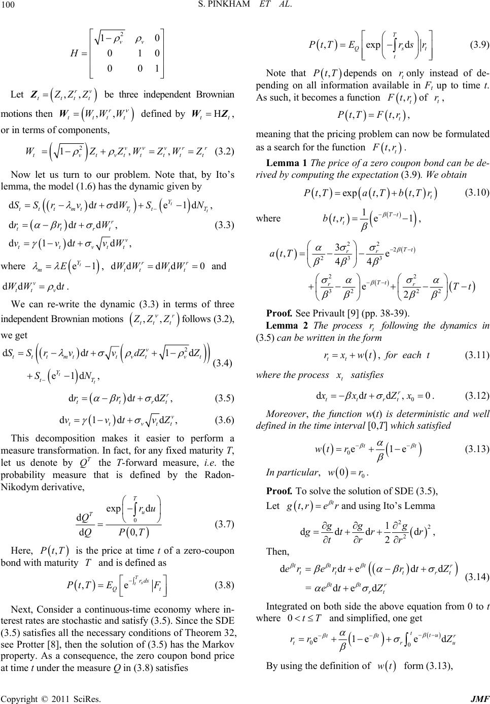 S. PINKHAM ET AL. 100 2 10 01 00 vv H 0 1 Let ,, rv tttt ZZZ tt WW be three independent Brownian motions then ,, r tt W W defined by tt WZ, or in terms of components, 2 1,, vvr tvt vttttt WZZWZW Z r (3.2) Now let us turn to our problem. Note that, by Ito’s lemma, the model (1.6) has the dynamic given by ddde ddd, d1d d, t tt Y tttmtT tT r ttrt v ttvtt SSrvtWSN rrtW vvtvW 1d, (3.3) where , and e1 t Y mE dd dd0 rr tt tt WW WW dd d v tt v WW t . We can re-write the dynamic (3.3) in terms of three independent Brownian motions ,, r tt t ZZ follows (3.2), we get 2 dd 1 e1d, t t v tttmttvt vt Y tT SSrvtv dZZ SN d d, t Z (3.4) dd r ttr rrt (3.5) d1d d v ttvt vvtv , t Z (3.6) This decomposition makes it easier to perform a measure transformation. In fact, for any fixed maturity T, let us denote by the T-forward measure, i.e. the probability measure that is defined by the Radon- Nikodym derivative, T Q 0 exp d d d0, T u Tru Q QPT (3.7) Here, is the price at time t of a zero-coupon bond with maturity and is defined as ,PtT T ,e T s trds Q PtT EF t (3.8) Next, Consider a continuous-time economy where in- terest rates are stochastic and satisfy (3.5). Since the SDE (3.5) satisfies all the necessary conditions of Theorem 32, see Protter [8], then the solution of (3.5) has the Markov property. As a consequence, the zero coupon bond price at time t under the measure Q in (3.8) satisfies ,expd T Qs t PtTEr sr t (3.9) Note that ,PtT depends on tonly instead of de- pending on all information available in Ft up to time t. As such, it becomes a function r , t tr of , t r ,, t PtT Ftr, meaning that the pricing problem can now be formulated as a search for the function ,t tr . Lemma 1 The price of a zero coupon bond can be de- rived by computing the expectation (3.9). We obtain ,exp,, t PtTatTbtT r (3.10) where 1 ,e Tt t btr 1 , 22 2 23 3 22 32 22 3 ,e 44 e2 Tt rr Tt rr atT Tt Proof. See Privault [9] (pp. 38-39). Lemma 2 The process t following the dynamics in (3.5) can be written in the form r tt rxwt, for each t (3.11) where the process t satisfies 0 ddd, r ttrt xxtZx 0 . (3.12) Moreover, the function w(t) is deterministic and well defined in the time interval [0,T] which satisfied 0e1e t wt r t (3.13) In particular, 0 0wr . Proof. To solve the solution of SDE (3.5), Let ,t tre r and using Ito’s Lemma 22 2 1 ddd d 2 gg g, tr r tr r Then, dded = ded ttt tt tr ttr rt erertrtZ et Z d r t (3.14) Integrated on both side the above equation from 0 to t where 0tT and simplified, one get 00 e1e ed ttu tt tr rr Z r u By using the definition of form (3.13), wt Copyright © 2011 SciRes. JMF 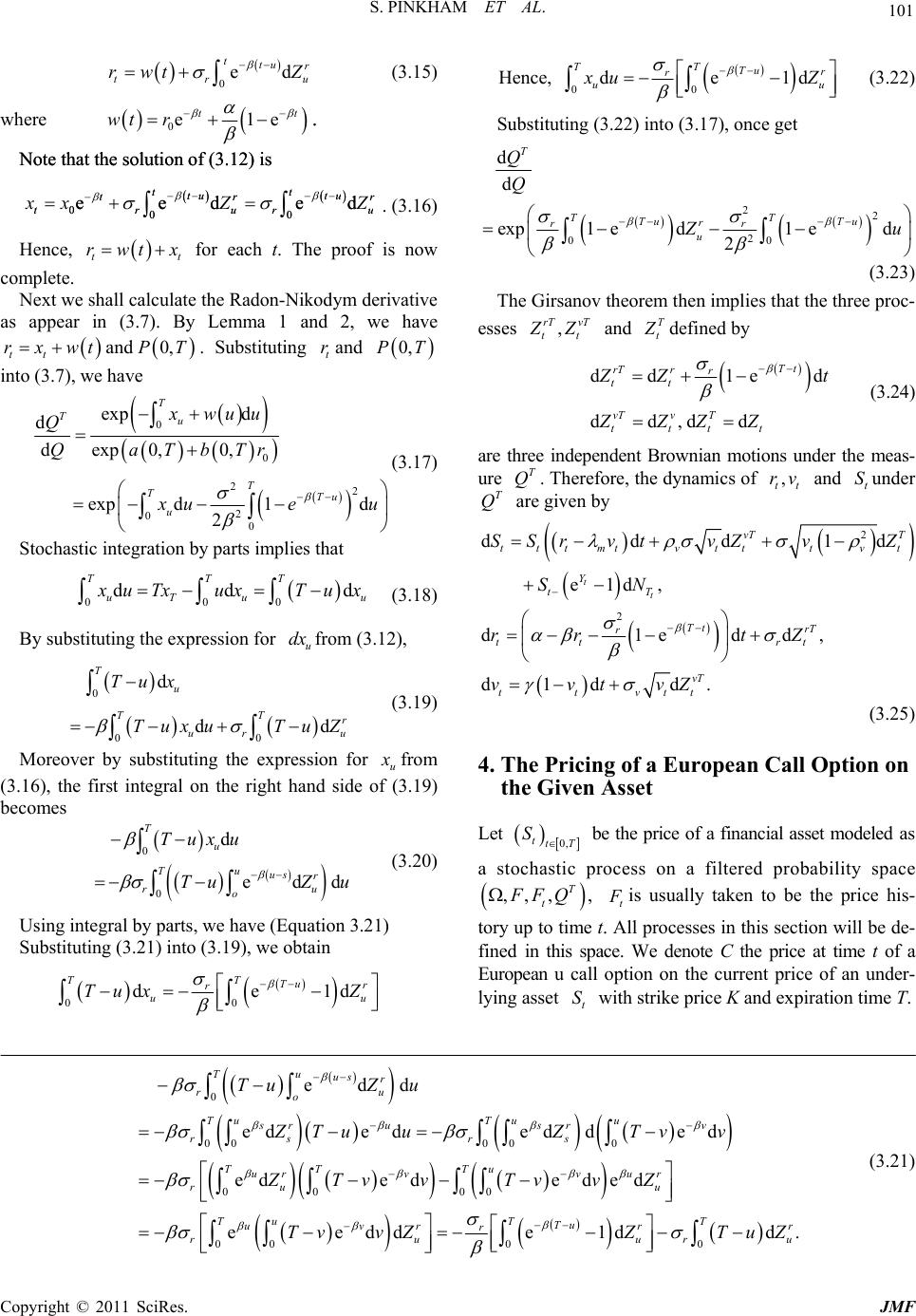 S. PINKHAM ET AL. Copyright © 2011 SciRes. JMF 101 uHence, 00 de1 TT Tu r r uu d uZ (3.22) 0ed ttu r tr rwtZ (3.15) where 0e1e tt wt r . Note that the solution of (3.12) is Note that the solution of (3.12) is 000 eede tt tu tu tr trur 000 eede tt tu tu tr trur d r u . d r u xZ Substituting (3.22) into (3.17), once get Z t . (3.16) 22 2 00 d d exp1 ed1 ed 2 T TT Tu Tu r rr u Q Q u Hence, for each t. The proof is now complete. t rwt x (3.23) Next we shall calculate the Radon-Nikodym derivative as appear in (3.7). By Lemma 1 and 2, we have and . Substituting and tt rxwt 0,PT t r 0,PT into (3.7), we have The Girsanov theorem then implies that the three proc- esses , rT vT tt Z and T t defined by 0 0 22 2 0 0 exp d d dexp 0,0, expd1d 2 T Tu T TTu u xwuu Q QaTbTr ue u d u dd 1e dd,dd Tt rTr r tt vTv T tttt d Zt ZZZZ (3.24) are three independent Brownian motions under the meas- ure . Therefore, the dynamics of and under are given by T Q, tt rv t S T Q (3.17) 2 2 ddd1 e1d, d1edd, d1d d. t t vT T tttmtv tttvt Y tT Tt rT r tt rt vT ttvtt SSrvtvZvZ SN rr tZ vvtvZ d (3.25) Stochastic integration by parts implies that 000 dd TTT uT u uTxuxTux (3.18) By substituting the expression for from (3.12), u dx 0 00 d dd T u TT r ur Tux Tuxu TuZ u (3.19) Moreover by substituting the expression for u from (3.16), the first integral on the right hand side of (3.19) becomes 4. The Pricing of a European Call Option on the Given Asset 0 0 d edd T u Tu us r ru o Tuxu TuZ u (3.20) Let 0, ttT S be the price of a financial asset modeled as a stochastic process on a filtered probability space ,, ,, T t FFQ t is usually taken to be the price his- Using integral by parts, we have (Equation 3.21) Substituting (3.21) into (3.19), we obtain 00 de1 TT Tu r r uu Tux Z d tory up to time t. All processes in this section will be de- fined in this space. We denote C the price at time t of a European u call option on the current price of an under- lying asset with strike price K and expiration time T. t S 0 0000 0 00 00 00 0 edd ede dedded ed ededed eedde1d Tu us r ru o TuTu u sr usrv rs rs TT Tu urvv ur ru u Tu T Tu uvr r r ruu TuZ u ZTuuZTv v ZTvv TvvZ Tv vZZ 0d. Tr ru TuZ (3.21) 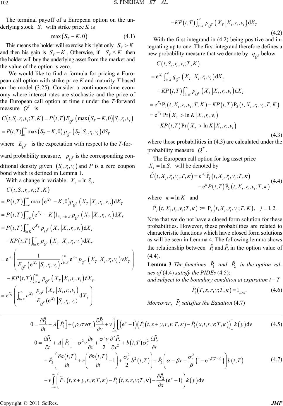 S. PINKHAM ET AL. 102 The terminal payoff of a European option on the un- derlying stock with strike price t S is max,0 T SK (4.1) This means the holder will exercise his right only and then his gain is T. Otherwise, if T T SK KSKS then the holder will buy the underlying asset from the market and the value of the option is zero. We would like to find a formula for pricing a Euro- pean call option with strike price K and maturity T based on the model (3.25). Consider a continuous-time econ- omy where interest rates are stochastic and the price of the European call option at time t under the T-forward measure is T Q 0 ,,,;,,max,0 ,, (, )max,0, ,d T T tt tTtt t Q TTtttT Q CtS rvTKPtTESKS rv PtTSKpSSr vS where is the expectation with respect to the T-for- T Q E ward probability measure, is the corresponding con- T Q p ditional density given and P is a zero coupon bond which is defined in Lemma 1. ,, tt t Srv With a change in variable ln, tt S ln ln ln ln ln ,,,;, ,maxe ,0,,,d ,e1 ,,d = ,e,,d ,,,d 1 ee e,, T T T T T T T T tT T T T tt t X TtttT Q X XKTtttT Q K X TtttT Q K Tttt T Q K XX TtttT QX K tt t Q CtS rvTK PtTKpXX rvX PtTKpXX rvX PtTpXX rvX KPtTpXXrvX pXXrvvX ESrv ,, ln ,,,d TTtttT Q K KPt TpXXrvX ln ,, ed (e,,) T tT T T Tttt Q XX T X K tt t Q pXXrv eX ESrv ln ,, TTtttT Q K,d PtTpXX rvX (4.2) With the first integrand in (4.2) being positive and in- tegrating up to one. The first integrand therefore defines a new probability measure that we denote by below T Q q ln ln ,,,;, e,,d ,, t T T tt t X TtttT Q K TtttT Q K CtS rvTK qXXrvX ,d PtTpXX rvX 12 eP, ,,;,, P,,,;, ePrln,, ,Prln,, t t X tt ttt t X Tttt Tttt tXrvTKKPtTtXrvTK XKXrv KPt TXKXrv (4.3) where those probabilities in (4.3) are calculated under the probability measure . T Q The European call option for log asset price ln tt S will be denoted by 1 2 ˆ,,,;, eP,,,;, e,P,,,;, t X tt ttt t tt t CtX rvTtX rvT PtTtX rvT (4.4) where ln and P,,,;, := P,,,;, , 1,2 jtttjttt tX rvTtX rvTKj . Note that we do not have a closed form solution for these probabilities. However, these probabilities are related to characteristic functions which have closed form solutions as will be seen in Lemma 4. The following lemma shows the relationship between and in the option value of (4.4). 1 P 2 P Lemma 3 The functions and in the option val- ues of (4.4) satisfy the PIDEs (4.5): 1 P 2 P and subject to the boundary condition at expiration t= T 1,,,;,1 . x PTxrvT (4.6) Moreover, satisfies the Equation (4.7) 2 P 11 111 0e1,,,;,,,, y vv PP ;,d PvvPtxyrvTPxtrvTkyy tv (4.5) 2 2 22 222 22 22 2( 22 2 22 0, 2 ,, 1, 1e 2 ,,,;,,,,;,(e1) d r Tt rr y PPP vv AP vbtT tx r x atT btT PrbtTPr b tt P vPt xyrvTPt xrvTkyy x ) , tT (4.7) Copyright © 2011 SciRes. JMF 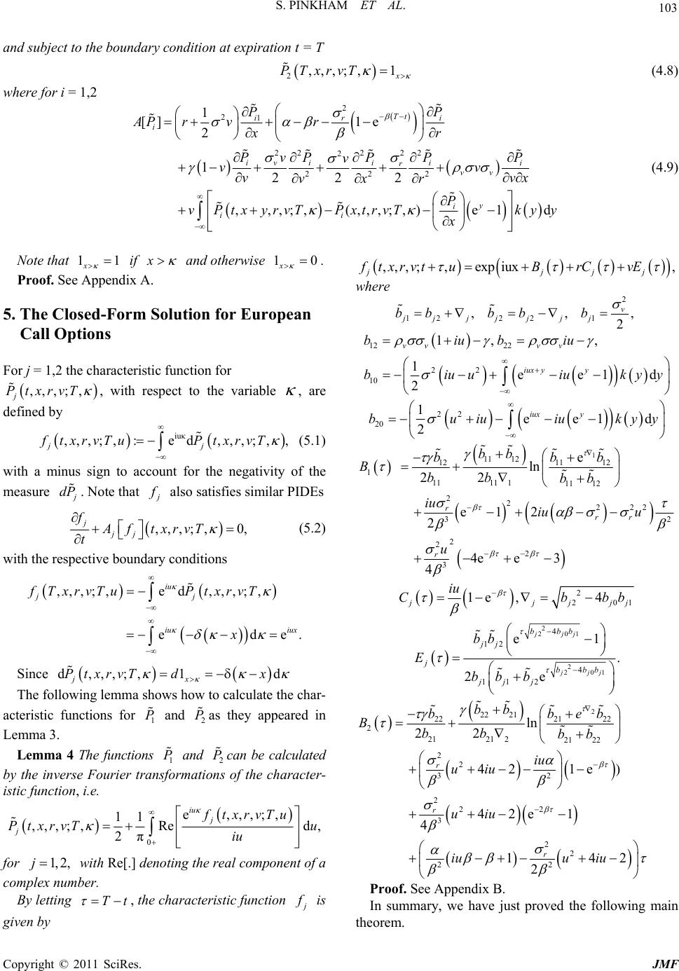 103 S. PINKHAM ET AL. and subject to the boundary condition at expiration t = T 2,,,;,1 x PTxrvT (4.8) where for i = 1,2 2 21 222 2 2 2 222 1 [] 1e 2 1222 ,,,; ,(,,,; , )e1d Tt ii r i iv iiii r vv y i ii PP AP rvr xr PvPP PP v vv vv vxr P vPt xyrvTPxt rvTkyy x x (4.9) Note that if 11 x and otherwise 10 x . Proof. See Appendix A. 5. The Closed-Form Solution for European Call Options For j = 1,2 the characteristic function for , with respect to the variable ,,,;, j PtxrvT , are defined by iuκ ,,,;,:e d,,,;,, jj ftxrvTuPtxrvT (5.1) with a minus sign to account for the negativity of the measure dP . Note that also satisfies similar PIDEs ,,,;, 0, j jj fAf txrvT t (5.2) with the respective boundary conditions ,,,;,e d,,,;, ede. iu jj iu iux fTxrvTuPtxrvT x Since d,,,;,1d jx PtxrvT dx The following lemma shows how to calculate the char- acteristic functions for and as they appeared in Lemma 3. 1 P 2 P Lemma 4 The functions and can be calculated by the inverse Fourier transformations of the character- istic function, i.e. 1 P 2 P 0 e,,,;, 11 ,,,;, Red, 2π iu j j ftxrvTu PtxrvT u iu for with Re[.] denoting the real component of a complex number. 1, 2,j By letting Tt , the characteristic function is given by ,,,; ,expiux, jjj ftxrvt uBrCvE j where 2 1222 1 ,, 2 v jjjj jjj bbbbb , 12 22 22 10 1, , 1ee1 2 vv vv iux yy biubiu biuuiukydy 22 20 1ee1d 2 iux y buiuiuk yy 1 11 12 1211 12 1 111111112 22222 32 2 2 2 3 e ln 22 e12 2 4e e3 4 r rr r bb bbb Bbb bb iu iu u u 2 201 1e ,4 jj jj iu Cb bb 2 201 2 201 4 12 4 11 2 e1 . 2e jjj jjj bbb jj jbbb jj j bb E bb b 2 22 21 2221 22 2 2121 221 22 2 2 32 2 22 3 2 2 22 ln 22 42 1e) 42e 1 4 14 2 r r r bb bbe Bbb bb iu uiu uiu iuu iu 2 b Proof. See Appendix B. In summary, we have just proved the following main theorem. Copyright © 2011 SciRes. JMF  S. PINKHAM ET AL. 104 Theorem 5 The value of a European call option of SDE (3.25) is 12 ,,,;, ,,,;,(,),,,;, tt t tttt ttt CtS rvTK SPtX rvTKPtTPtXrvT where 1 and 2 are given in Lemma 4 and ,PtT is given in Lemma 1. 6. Acknowledgements This research is (partially) supported by The Center of Excellent in Mathematics, the commission on Higher Education (CHE). Address: 272 Rama VI Road, Ratchathewi District, Bangkok, Thailand. 7. References [1] P. Carr and L. Wu, “Time Change Levy Processes and Option Pricing,” Journal of Financial Economics, Vol. 17, No. 1, 2004, pp. 113-141. doi:10.1016/S0304-405X(03)00171-5 [2] R. C. Merton, “Option Pricing when Underlying Stock Returns are Discontinuous,” Journal of Financial Eco- nomics, Vol. 3, No. 1-2, 1976, pp. 125-144. doi:10.1016/0304-405X(76)90022-2 [3] D. Bates, “Jump and Stochastic Volatility: Exchange Rate Processes Implicit in Deutche Mark in Option,” Review of Financial Studies, Vol. 9, No. 1, 1996, pp. 69-107. doi:10.1093/rfs/9.1.69 [4] G. Yan and F. B. Hanson, “Option Pricing for Stochastic Volatility Jump Diffusion Model with Log Uniform Jump Amplitudes,” Proceeding American Control Conference, Minneapolis, 14-16 June 2006, pp. 2989-2994. [5] Y. J. Kim, “Option Pricing under Stochastic Interest rates: An Empirical Investigation,” Asia Pacific Financial Markets, Vol. 9, No. 1, 2001, pp. 23-44. doi:10.1023/A:1021155301176 [6] D. Brigo and F. Mercuiro, “Interest Rate Models: Theory and Practice,” 2nd Edition, Springer, Berlin, 2001. [7] R. Brummelhuis, “Mathematical Method for Financial Engineering,” University of London, 2009. http://www.ems.bbk.ac.uk/for_students/msc./math_metho ds/lecture1.pdf [8] P.E. Plotter, “Stochastic Integration and Differential Equation,” Stochastic Modeling and Applied Probability, Vol. 21, 2nd Edition, Springer, Berlin, 2005. [9] N. Privault, “An Elementary Introduction to Stochastic Interest Rate Modeling,” Advance Series on Statistical Science & Applied Probability, Vol. 2, World Scientific, Singapore, 2008. [10] M. G. Kendall, A. Stuat and J. K. Ord, “Advance Theory of Statistics Vol. 1,” Halsted Press, New York, 1987. Copyright © 2011 SciRes. JMF 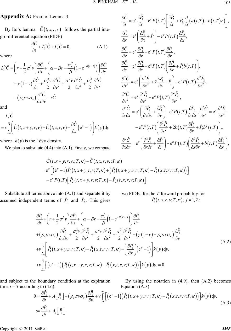 S. PINKHAM ET AL. 105 Appendix A: Proof of Lemma 3 By Ito’s lemma, follows the partial inte- gro-differential equation (PIDE) ˆ,,,Ctxrv ˆˆˆ 0, DJ tt CLC LC t (A.1) where 2 2 22 222 2 22 2 ˆˆ 1 ˆ1e 2 ˆˆˆ 1222 ˆˆ Tt Dr t vr vv CC LC rvr 2 ˆ r v CCvCC vvvxr C vrC xv and ˆ ˆ ˆˆ ,,,,,,e1 d J t y LC C vCtxyrvCtxrvk yy x where is the Lévy density. ()ky We plan to substitute (4.4) into (A.1). Firstly, we compute 12 2 12 1 12 12 2 2 2 11 1 22 ˆ ee,, , ˆ ee,, ˆ ee,, ˆ ee, ,, ˆ e2e x x x x x PP CPtTPatTbtTr tt tt PP CPPtT xx x PP CPtT vvv PP CPtT PbtT rrr PP CPPt x xx , 2 2 2 22 2 12 22 2 2 22 1121 22 2 2 22 2 2 ,, ˆ ee,, ˆˆ ee,,e e, 2,,,. x xx P Tx PP CPtT vv v PPPP CC PtT vxvxvvx rr PP PtTbtTPb tT r r 22 2 112 2 ˆ ee,, xPPP P CPtTbtT , rxrrxrx 111 22 ˆˆ ,,,,;,,,,,;, ee1,,,;,,,,;,,,,;, e(,),,,;,,,,;, . xy Ctxyrv TCtxrv T PtxyrvTPt xyrvTPxtrvT PtTPt xyrvTPt xrvT Substitute all terms above into (A.1) and separate it by assumed independent terms of 1 and 2 . This gives two PIDEs for the T-forward probability for ,,,;, ,1,2: i PtxrvTj 2 2 11 1 22222 2 1111 222 1 11 11e 2 1 222 ,,,;,,,,;,e1d. e Tt r vr vv vv y y PP P rv r tx r v PPPP v vv vx v vxr P vPtxyrvTPxtrvTkyy x v 1 P v 11 1,,,;,,,,;,d.0Ptx yrvTPxtrvTky y (A.2) and subject to the boundary condition at the expiration time t = T according to (4.6). By using the notation in (4.9), then (A.2) becomes Equation (A.3) 11 111 1 11 0e1,,,;,,,, :. y vv PP ;,d. PvvPtxyrvTPxtrvTkyy tv PAP t (A.3) Copyright © 2011 SciRes. JMF 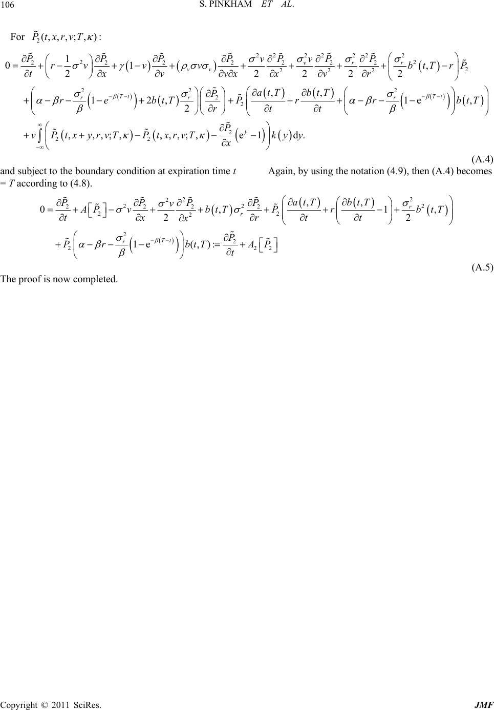 S. PINKHAM ET AL. 106 For 2(,, , ;,):PtxrvT 2 22222 2 2 2 2222222 2 222 22 2 2 2 1 01 , 22222 ,, 12, 1e 2 vrr vv Tt Tt rr r v PPPPPPP v rvv vbtTrP txvvx xvr atT btT P re btTPrr rtt 2 22 , ,,,;,,,,;,e1d. y btT P vP txyrvTPtxrvTkyy x Again, by using the notation (4.9), then (A.4) becomes (A.4) and subject to the boundary condition at expiration time t = T according to (4.8). 2 2 2 22 2222 22 2 2 2 222 ,, 0, 22 1e (,): r r Tt r atT btT PPPP v2 1, PvbtT PrbtT tx rtt x P PrbtT AP t (A.5) The proof is now completed. Copyright © 2011 SciRes. JMF  107 S. PINKHAM ET AL. Appendix B: Proof of Lemma 4 To solve the characteristic function explicitly, letting Tt 1 f be the time-to-go, we conjecture that the func- tion is given by 1 111 ,,,;, exp iux, ftxrvtu BrCvE (B.1) and the boundary condition 111 000BCE0. This conjecture exploits the linearity of the coefficient in PIDEs (5.2). Note that the characteristic function of 1 always exists. In order to substitute (B.1) into (5.2), firstly, we compute f 1 1111 ,, f BrCvEfiuf t 2 2 11 1 11 111 2 22 22 11 111 1 22 22 11 11 11 1 11 ,, ,, ,, e(,,,; ,) (,,,;,)(,,,; ,) iux fff Cf Efuf rvx ff EfCf vr ff iuC fiuE f xr vx ftxrvt u ftx yrvtuftxrvtu , 1 1 f x Substituting all the above terms into (5.2), after can- celling the common factor of 1 , we get a simplified form as follows: 11 22 22 111 22 2 1111 0 1ee1 e1ed 22 +1e 2 iuxyy iux v vv Tt rr rCiu C vEiuEEiuuiuk yy BCCE By separating the order, r, v and ordering the re- maining terms, we can reduce it to three ordinary differ- ential equations (ODEs) as follows: 11 ()() ,CCiu (B.2) 2 2 11 1 2 2 1 2 ee1d, 2 v vv iux yy EE iuE iuuiukyy (B.3) 22 2 1111 C1e . 2 Tt rr BCE (B.4) It is clear from (B.2) andthat (0)0C 11e , iu C (B.5) Let 2 1, 2 v b 21, vv biu 22 0 1ee1 2 iux yy biuuiuky dy and substitute all term above into (B.3). we get 22 22 0122 01 111 1 11 44 22 bb bbbb bb EbE E bb By method of variable separation, we have 1 1 22 22 0122 01 11 11 dd 44 22 Eb bb bbbbbb EE bb Using partial fraction on the left hand side, we get Copyright © 2011 SciRes. JMF  S. PINKHAM ET AL. 108 1 22 11 11 11 dd () 22 E bb EE bb where 2 20 4bbb1 . Integrating both sides, we have 2 1 1 0 2 1 1 2 ln 2 b Eb b Eb Using boundary condition1(0)0E we get 2 0 2 ln b Eb Solving for1()E , we obtain 12 1 11 2 e1 2e bb E bb b (B.6) where . 12 22 ,bb bb In order to solve1()B explicitly, we substitute 1()C and 1()E in (B.5) and (B.6) into (B.4) . 22 2 122 2 212 2 2 11 2 '1ee e1 12ee 22e rr r iu iu iu B bb u bb b Integrating with respect to and using boundary con- dition 1(0)B0 , then we get 222 12 2 22 22 33 12 212 11 12 2 e14ee 3 24 e ln 22 rr rr Biu u iu u bb bbb bb bb The details of the proof for the characteristic function 2 are similar to1 . Hence, we have 2 222 ,,,;, exp ftxrvT u iux BrCvE where 22 ,BC and 2()E are as given in this Lem- ma. We can thus evaluate the characteristic function in close form. However, we are interested in the probabil- ity P . These can be inverted from the characteristic functions by performing the following integration iuκ 0 ,,,;, e,,.;, 11Re d 2 j j PtxrvT ftxvrTuu iu e for 1, 2j where ln tt S and ln , see Ken- dall et al. [10]. The proof is now complete. Copyright © 2011 SciRes. JMF
|