Journal of Mathematical Finance, 2011, 1, 63-71
doi:10.4236/jmf.2011.13009 Published Online November 2011 (http://www.SciRP.org/journal/jmf)
Recent Developments in Option Pricing
Hui Gong1, Aerambamoorthy Thav aneswaran2, You Liang2
1Department of Mat hemat i c s & Computer Science , Valparaiso University, Valparaiso, USA
2Department of Stat i s t i c s, University of Manitoba, Winnipeg, Canada
Received September 1, 2011; revised S e p tember 28, 2011; accepted October 10, 2011
Abstract
In this paper, we investigate recent developments in option pricing based on Black-Scholes processes, pure
jump processes, jump diffusion process, and stochastic volatility processes. Results on Black-Scholes model
with GARCH volatility (Gong, Thavaneswaran and Singh [1]) and Black-Scholes model with stochastic
volatility (Gong, Thavaneswaran and Singh [2]) are studied. Also, recent results on option pricing for jump
diffusion processes, partial differential equation (PDE) method together with FFT (fast Fourier transform)
approximations of Pillay and O’ Hara [3] and a recently proposed method based on moments of truncated
lognormal distribution (Thavaneswaran and Singh [4]) are also discussed in some detail.
Keywords: Stochastic Volatility, Black-Scholes Partial Differential Equations, Option Pricing, Monte Carlo
1. Introduction
Option pricing is one of the major areas in modern fi-
nancial theory and practice. Since Black, Scholes, and
Merton introduced their path-breaking work on option
pricing, there has been explosive growth in derivatives
trading activities in the worldwide financial markets. The
main contribution of the seminal work of Black and
Scholes [5,6] and Merton [7] was the introduction of a
preference-free option pricing formula that does not in-
volve an investor’s risk preferences and subjective views.
Due to its compact form and computational simplicity,
the Black-Scholes formula enjoys great popularity in the
finance industries and is based on the strong assumption
that the volatility of the stock returns is constant. How-
ever, implied volatility of the stock prices suggests sto-
chastic volatility models are more appropriate to model
the stock price. The most popular approach is to use the
Heston model (Heston [8,9]), which assumes that the
underlying asset follows the Black-Scholes model but the
volatility is stochastic and follows the Cox Ingersoll Ross
process (Cox, Ingersoll and Ross [10]). The empirical
results of Bakshi, Cao and Chen [11] suggest that taking
stochastic volatility into account is important in option
pricing. Motivated by the theoretical considerations, Scott
[12], Hull and White [13,14], Ritchken and Trevor [15],
and Wiggins [16] generalized the Black-Scholes model
to allow stochastic volatility.
Heston and Nandi [17] first provided a solid theoretical
foundation based on the concept of locally risk-neutral
valuation relationship for option valuation under nonlin-
ear GARCH models using characteristic functions. Heston
and Nandi [17], Elliot, Siu and Chan [18], Christoffersen,
Heston and Jacobs [19], and Mercuri [20] among others
derived clo sed form option pricing formula unde r various
GARCH models. Recently, Badescu and Kulpeger [21],
Barone-Adesi et al. [22,23], and Gong, Thavaneswaran
and Singh [1] including others have studied option pric-
ing under GARCH volatility. Thavaneswaran, Peiris and
Singh [24] and Thavaneswaran, Singh and Appadoo [25]
studied option pricing using the moment properties of the
truncated lognormal distribution. Gong, Thavaneswaran
and Singh [1,2] studied Black-Scholes models with
GARCH volatility and with stochastic volatility as in Taylor
[26]. They carried out extensive empirical analysis of the
European call option valuation for S & P 100 index and
showed that the proposed method outperformed other
compelling stochastic volatility pricing models. In Tha-
vaneswaran and Singh [4], option pricing for jump diffu-
si on process with stochastic volatility was studied by view-
ing option pricing as a truncated moment of a lognormal
distribution. Pillay and O’ Hara [3] studied the FFT based
option pricing under a mean reverting process with sto-
chastic volatility and ju mps by using the PDE approach.
In this paper, we first derive the Black Scholes partial
differential equation for stochastic volatility models and
then obtain closed-form solutio ns for the resulting PDEs.
The rest of this paper is organized as follows. In Section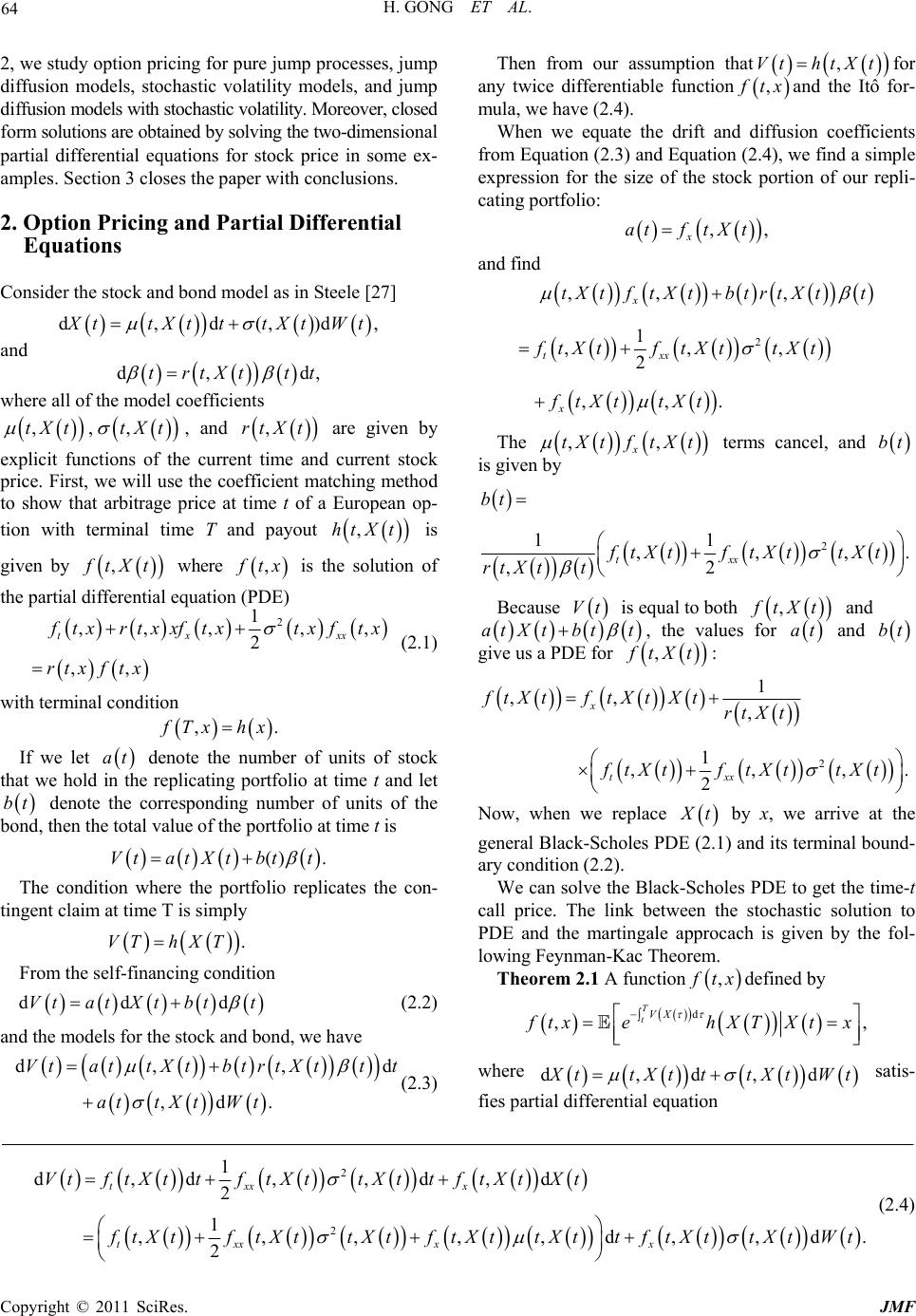

H. GONG ET AL.
64
,
2, we study option pricing fo r pure jump processes, ju mp
diffusion models, stochastic volatility models, and jump
diffusion models with stochastic volatility. Moreover, closed
f or m so lu t io n s ar e ob t a ined by solving the two -dimensi onal
partial differential equations for stock price in some ex-
amples. Section 3 closes the paper with conclusions.
2. Option Pricing and Partial Differential
Equations
Consider the stock and bond model as in Steele [27]
    
d,d(,)d  
X
ttXtttXtWt
and


  
d,  trtXt ttd,
where all of the model coefficients



,tXt  ,, and are given by
explicit functions of the current time and current stock
price. First, we will use the coefficient matching method
to show that arbitrage price at time t of a European op-
tion with terminal time T and payout
 
,tXt 
   
,rtXt

 
,htXt is
given by
 
,
f
tXt where

,
f
tx is the solution of
the partial differential equation (PDE)
 

2
1
,,, ,,
2
,,
tx xx
f
txrtxxftxtx ftx
rtxf tx
 

(2.1)
with terminal condition

,.fTxhx
If we let denote the number of units of stock
that we hold in the replicating portfolio at time t and let
denote the corresponding number of units of the
bond, then the total value of the portfolio at time t is

at

bt
 
() .VtatXt btt  
The condition where the portfolio replicates the con-
tingent claim at time T is simply
  
VT hXT

d
.
From the self-financing condition
 
ddd  Vtat Xtbtt (2.2)
and the models for the stock and bond, we have
      

   
d,,
,d.




VtattXtbtrtXttt
attXt Wt(2.3)
Then from our assumption that


 
,htXt

,
Vt for
any twice differentiable function
f
txand the Itô for-
mula, we have (2.4).
When we equate the drift and diffusion coefficients
from Equation (2.3) and Equation (2.4), we find a simple
expression for the size of the stock portion of our repli-
cating portfolio:

 
,,
x
ttaf

X
t
and find







   


 




   
2
,, ,
1
,,,
2
,,.
x
txx
x
tXtf tXtbtrtXtt
ftXtf tXttXt
ftXttXt






The








,,
x
tXtftXt 
terms cancel, and


bt
is given by


   





2
11
,,,
2
,txx
bt
f tXtftXttXt
rtXtt







.
Because


Vt is equal to both
 
,

f
tXt and








atXt tbt  , the values for at and



bt
give us a PDE for




,
f
tXt :
     

     
2
1
,, ,
1
,,,
2
x
txx
ftXtf tXtXtrtXt
f tXtftXttXt 





.
Now, when we replace

X
t by x, we arrive at the
general Black-Scholes PDE (2.1) and its terminal bound-
ary condition (2.2).
We can solve the Black-Scholes PDE to get the time-t
call price. The link between the stochastic solution to
PDE and the martingale approcach is given by the fol-
lowing Feynman-Kac Theorem.
Theorem 2.1 A function

,

f
txdefined by

 
  
d
,,
T
tVX
f
txehXTX tx
 








where





  


d,d,d  
X
ttXtttXtWt
satis-
fies partial differential equation
         
 













2
2
1
d,d,,d ,d
2
1
,,,,,d,,d
2
txx x
txxxx
VtftXt tftXttXt tftXt Xt
.
f
tXtftXttXtftXttXttftXttXtWt

 
 

 


(2.4)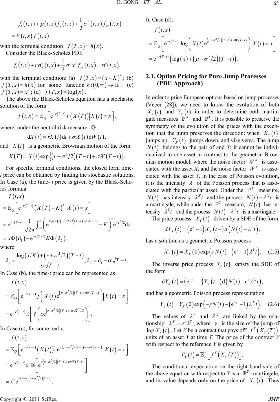

65 H. GONG ET AL.
 

2
1
,,, ,,
2
,,
tx xx
f
txtx ftxtx ftx
Vtxftx
 

with the terminal condition


,.
f
Tx hx
oles PDE Consider the Black-Sch
 
22
1
,, ,
2
txxx ,,
f
txrxftxxftxrftx   
with the terminal condition: (a)
 
,
f
Tx Kx



:0,h
; (b)
; (c)

,Tx hxfor some function

,
f
f
Tx x

; (d)
 
,log
f
Tx x.
holes equation has a stochastiThe above the Black-Scc
solution of the form






,e
rT t,
f
txX tx



where, undereutral risk measu
f XT





the nre 
 
ddd,  
,
X
trXtt XtWt
and


X
t is a geometric Brownian motion of the form
 

 

22exp .
X
TXtrTt WTt   
For specific terminal conditions, the closed form time-
se (a
les formula
t price can be obtained by finding the stochastic solutions.
In Ca), the time- t price is given by the Black-Scho-



  
 


 
2 2log 2
()
12
,
e ed
2
de d,
xr Tt Ttzz
rT t
ftx
2
e
1
e
rT t
Q
rT t
XT KXtx
K
z
xK
   






 

where














2
12
log
d,d
2. xKrT tTt
Tt


 
1 d

In Case (b), the time-t price can be represented as





 




22
ee
ee .
Tt WTt
rT t
Q
x
22rT
tTtZ
rT t
,ft
f
XXx
fx
tt
  














In Case (c), for some real v,
  
 



 
 



 



2
2
2
12
(
,
ee
e.
rT tT tWT t
Q
WTt
rTt
ftx
22
ee
rT t
rT t
X
tXtx
x
x
 



 

 








In Case (d),


 
 
 








 






22
2
,
elog e
eog 2l.
TtWTt
rT t
Q
rT t
ftx
Xt tX
tx
x
T
 
















2.1. Option Pricing for Pure Jump Processes
(PDE Approach)
In order to price Eu ropean op tion s based on jump processes
we need to know the evolution of both (Vecer [28]),


Y
X
t and


X
Yt
X

he ev
jump
in order to determine both martin-
asures and . It is possible to preserve the
ry of tolution of the prices with the excep-
preserves the direction: when
gale me
symmet
tion that the
Y



Y
X
t
jumps up,


X
Yt jumpn, and vise versa. Ts dowhe jump


Nt
ualized
ated w
bele pair and Y; it cannot be indi
tnrast to the geom
it Y. case of Poiss
on
o
h t
gs to th
one asset i
he asset
of
cont
In the
vi-
etric Brow-
olution,
d
nian motion model, where the noise factor X W is asso-
ciated with the asset X, and the noise factor Y W is asso-
ci on ev
it is the intensity

of the Poisson process that is asso-
ciated with the particular asset. Under the X  measure,


Nt has intXtensity

and the process

X
Nt t

 is
a marting ale, wunder Y  measure, hile the


Nt has in-
tensity Yt

and the process

Y
Nt t

 is a martingale.
The price process


Y
X
t driven by a SDE of the form




 

e1 ,
Y
YY
dXXtd Nt

 
has a solution as a geometric Poisson process
 

tt


0expe 1.

 
YY
XX Ntt (2.5)
The inverse price process

X
Yt satisfy the SDE of
the form
 t
Y




 

de de,
 
 
XX
YYttNtt
and has a geometric Poisson pess representation


roc
1 
X




0e 1.
X
XX
YY Nttt



 (2.6) exp
Y

and X

The values of are linked by the rela-
tionship e
XY 

 , where

is the size of the jump of


log Y
X
t. Let V be a contract that pays off




YY
f
XT
the conunits of an asset Y at time e price of
with respect to the reference Y is given by
T. Thtract V

 
.
YY
Vft

Yt Y
XT





The conditional expectation on the right hand side of
the above equation with respect to Y is a martingale,
Y

and its value depends only on the price of


Y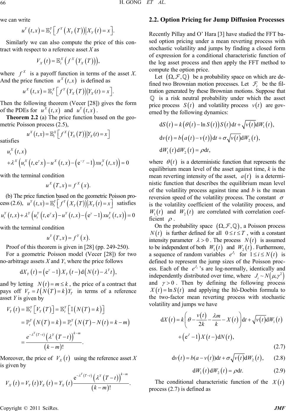
X
t. Thus

H. GONG ET AL.
66
we can write


  
,.
Y
utxfXT Xtx


Similarly we can also comute the price of this con-
respect to a reference asset X as

 
,
XX
Xt X
VftYT
YYY
tY

p
tract with
where X
f
is a payoff function in terms of the asset X.
And the price function is defined as
  

,
X
utx
,(.
XXY
tXX
utxfYTYt x




Then the following theorem (Vecer [28]) ge form
of the PDEs fo
)
ives th
r and
Theorem 2.2ice sed one geo-
metric Poisson pr

,
X
utx
(a) The pr

,
Y
utx.
function ba th
ocess (2.5),
  
,()
XXX
tXX
utxf YTYtx




satisfies 

 
,
X
t
utx
u



with the terminal condition
nction bathe geomric Poisson pro-
ce
,e ,e 1,0
XX X X
tx
txu txxu tx




 
,.
XX
uTxf x
(b) The price fused on et
s s (2.6),
 


,
YYY
tYY
utxfXTXtx



 satisfies




,,e,
YYY Y
utxutxut

 



e1,
Y
tt x
x xutx



0
erminal condition
Proof of this theorem is given in [28] (pp. 249-250).
For a geometric Poisson model (Vecer [28]) for two
where the price follows
,
with the t
 
,.
YY
uTxf x
no-arbitrage assets X and Y,




de1d

  
Y
YY

X
tXtNt t
an in terms of a
asset Y is
d by letting

Ntm k, the price of a contract that
pays off VI reference
 
TT
TN k
n by Y give
 




 





.
!km

Ykm
Tt Y
eT t



 
YY
YY
tt
VtVTNT k
NTkNTNtk m

  

 


Moreover, the price of using the reference asset X
is given by
Yt Y t




X
Vt
 



 
e.
Ykm
Tt Y
XYX
tTt VVYt



 

!
X
Yk ttm 
2.2. Option Pricing for Jump Diffusion Processes
Recently Pillay and O’ Hara [3] have studied the FFT
sed option pricing under a mean reverting process with
stochastic volatility and jumps by finding a closed form
of expression for a conditional characteristic function of
the log asset process and then apply the FFT method to
e.
ba-
compute the option pric
Let


,,
row
enerated b
a risk neutral
be a probability space on which are de-
fined two Bnian motion processes. Let be the fil-
tration gy these Brownian mose th
is probability under which the asset
t

tions. Suppoat

price process


St and volatility process

vt are gov-
rned by the following dynamics: e
 



 

 

1
2
12
dlndd,
ddd,
dd d,



 
 

Sk SStvW
vba
tttt tt
ttt tt
t
v
Wt
vt W
Wt
where


t 
is a deterministic function that represents the
equilibrium mean level of the asset against time, k is the
mean reverting intensity of the asset,

at is a determi-
nistic function that describes the equilibrium mean level
of the volatility process against time and b is the mean
reversion speed of the volatility process. Thnstant e co

is the volatility coefficient of the volatility process, and


1
Wt and


2
Wt are correlated with correlation coef-
ficient

.
On the probability space , a Poisson process

,,


Nt
in is further defined for with a constant tensity parameter all 0tT , 0

. The process

Nt is assumed
pendeto be indent of both

1
Wt and

2
Wt
. Furthermore,
a sequence of random variables i
J
e for


1iNt is
defined to represent the jump sizes of the Poisson proc-
ess. Each of the i
J
e’s are log-normally, identically and
independently distributed over time, where


2
~,
i
JN


and 0

. Then by defining the following process




lnXt tS and applying the Itô-Doebin formula to
the two-factor mean reverting process with stochastic
volatility and s we have jump




 
1
d
2
e1 ,
J
t
t tt
v
Xk tvW
kk
Xt t



 



(2.7)
 

dd
d
t
mX
N



2
d()d d,   tt tvbvtvWt (2.8) a


12
dd d.ttWW t

 (2.9)
The conditional characteristic function of the


X
t
process (2.7) is defined as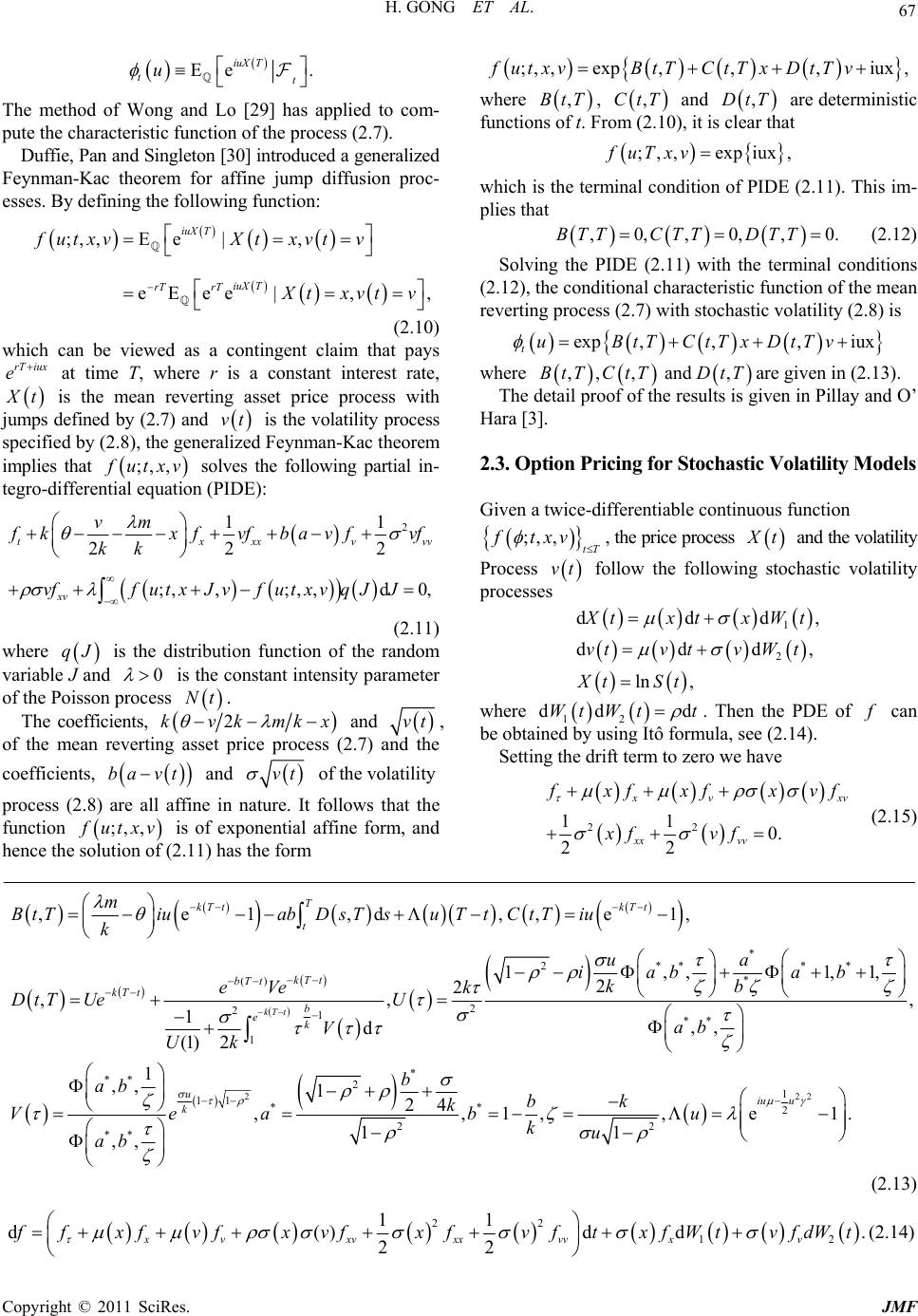

H. GONG ET AL.
67


Ee
tu



.
iuX
t
T

The method of Wong and Lo [29] has applied to com-
pute the characteristic function of the process (2.7).
Duffie, Pan and Singleton [30] introduced a generalized
Feynman-Kac theorem for affine jump diffusion proc-
esses. By defining the following function:





 


exp ,,,iux;, ,,fBtTCtTxDuv txTvt
where


,


,CtT


 


;, ,Ee|,
eEee |,,







iuX
iuX rrT
T
TT
tt
tt
futxvXxvv




X
xv v
(2.10)
contingent claim that pays
at time T, where r is a constant interest rate,
which can be viewed as a
rT iux
e

X
t is the mean reverting asset price process with
jumps defined by (2.7) and


vt is the volatility process
specified by (2.8), the generalized Feynman-Kac theorem
implies that

;,,
f
utxv solves the following partial in-
tegro-differential equation (PIDE):

  
2
1
22
;,,;,,d0,
txxx

1
2
v
xv
vm vv
f
kxfvfbavfv
kk
vffutxJvfutxvqJJ


 



 


 

variab
f 
(2.11)
where

qJ is the distribution function of the random
le J and 0

 is the constant intensity parameter
Poisson process

Nt.
The coefficients,
of the

kv mkx    and

2kvt ,
of the mean reverting asset price process (2.7) and the
coefficients,
 
ba vt and
 
tv  of the volatility
process (2.8) are all affine in nature. It follows that the
function

;, ,
f
utxv
solution of (is of exponential affine form, and hence the 2.11) has the form
,BtT and Dt are deterministic

,T

functions of t. From (2.10), it is clear that


;,, expiux,Txv
which is the terminal condition of PIDE (
fu
2.11). This im
plies that -




, ,,0.T TTT0, 0,BT CDT

 (2.12)
Solving the PIDE (2.11) with the terminal conditions
(2.12), the conditional characteristic function of the mean
reverting process (2.7) with stochastic volatility (2.8) is



 


exp ,,,iuxBtTC tTxDtTv 
tu




,,, and ,BtT CtTDtT where

are given i
2.3. Option Pricing for St ochastic Vol atility Models
twice-differentiable continu
n (2.13).
The detail proof of the results is given in Pillay and O’
Hara [3].
Given aous function


 
;, ,ftxv 
tT

, the price process

X
t and the volatility
rocess


vt follow the following stochastic volatility P
processes





1
ddd  XtWtx xt
X

,

2
dd d,  vt Wtv vt

ln ,tSt




dd dttWW t where 12

. Then the PDE of f can
be obtained by using Itô formula, see (2.14).
Setting the drift term to zero we have




x
 
0.
22
11
22
vxv
xx
fxfxf xvf
xf




 (2.15)
vv
vf 



 



 





*
2** **
*
2
21**
1
*
,e1,d,,e1,
1,,1,1,
2 2
, ,
1,,
(1) 2
,
kT t
T
kTt
t
b
ek
m
BtTiuabDsTsT t CtTiu
k
ua
iabab
kb e k
U
ab
V
Uk
a
V

kT t
()
,
kT t
bT t
kT tV
e
DtTUe
d
u




 

 





 



 





















222
*
*21
11 ** 2
22
**
1
,124
,,1,,e1.
11
,,
uiu u
k
b
bbk
k
ea b
ku
ab
u
 





 
  
 

 


 



(2.13)
 
22
12
11
d()dd
22

   

 

x vxvxxvvxv
fff fxv xxvxtvvffftf WfdtW. (2.14)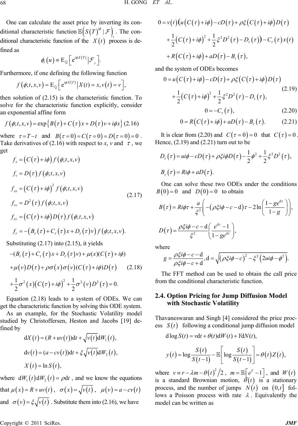

H. GONG ET AL.
68
One can calculate the asset price by inverting its con-
ditional characteristic function. The con-
ditional characteristic function


|
i
t
ST


of the

X
t process is de-
fined as


Ee.
iXT
tt
u





Furthermore, if one defining the following function



;, ,Ee(),,
iXT
f
txvXt xvt v







then solution of (2.15) is the characteristic function. To
solve for the characteristic function explicitly, consider
an exponential affine form
 

;, ,exp
f
txvBCxDv ix

  (2.16)
where Tt


and






000BCD   0
.
Take derivatives of (2.16) with respect to x, v and

, we
get
  
x
v
fC iftxv
f
  
 

 


 
2
2
;,,
;, ,
;, ,
;,,
vv
Dftxv
fC iftxv
fD ftxv
  


;, ,
;, ,.
xv
fC iDftxv
xx
f
BCxDvftxv
 
    
 
 
 

 



(2.17)
Substituting (2.17) into (2.15), it yields
 
 
    
2
222
()()()
11
0.
22
BC DvxCi
xC ivD
 
()
x
vDxv CiD




 .18)


 
 
(2
Equation (2.18) leads to a system of ODEs. We can
get the characteristic function by solving this ODE system.
As an example, for the Stochastic Volatility
studied by Christoffersen, Heston and Jacobs [1
fined by
model
9] de-

 
 
ln ,
1
2
d()d d,
d( )dd,
X
tRuvttvtWt
vtacvttvtWt 
 
 
where d
Xt St
 
12
dd

Wt Wtt,
 





  




 
   
222
0
11
22
,
(
)
vt uCicDCiD
CiD DCx
RCi aDB


t


 
 

 

and the system of ODEs becomes











 
222
0
11 ,
22
uC icDC iD
CiD D







 
 
 (2.19)

0,C


 (2.20)



  
0.RCiaDB


  (2.21)
It is clear from (2.20) and


00C  
that


0C 

.
Hence, (2.19) and (2.21) turn out to be
 
 
222
11 ,
22
.
DuicD iDD
BRiaD




 
 

One can solve these two ODEs under the conditions


00B

and


00D

to obtain
 
d 

and we know the equations
that
x
Ruvt,



x
vt, 



vacvt  
and
 
vvt  . Substit ute them into (2 .16), we have
2
1
d2ln ,
1
age
Ri icg
 



  







d
2d
d1
,
1
B
ic e
Dge


 


 



where


222
d,d2 .
d
ic
gic
ic ui



 
 





FFT method can be
the conditional characteristic function.
Option Pricin
with Stochastic Volatility
Thavaneswaran and Singh [4] considered the price proc-
ess
The used to obtain the call price
from
2.4. g for Jump Diffusion Model


St following a conditional jump diffusion model
 
   
dlog()d()d()d(),
log log
St S
yt ,
11
StvttWtYNt
ttZt
St St








where






22vrmt
  , 1
Y
me






Wt , and
is a standard Brownian mois a sta
process, and the number of jtion,

t 
umps

Nt ontionary


0,t fol-
lows a Poisson process with rate

. Equivalently the
model can be written as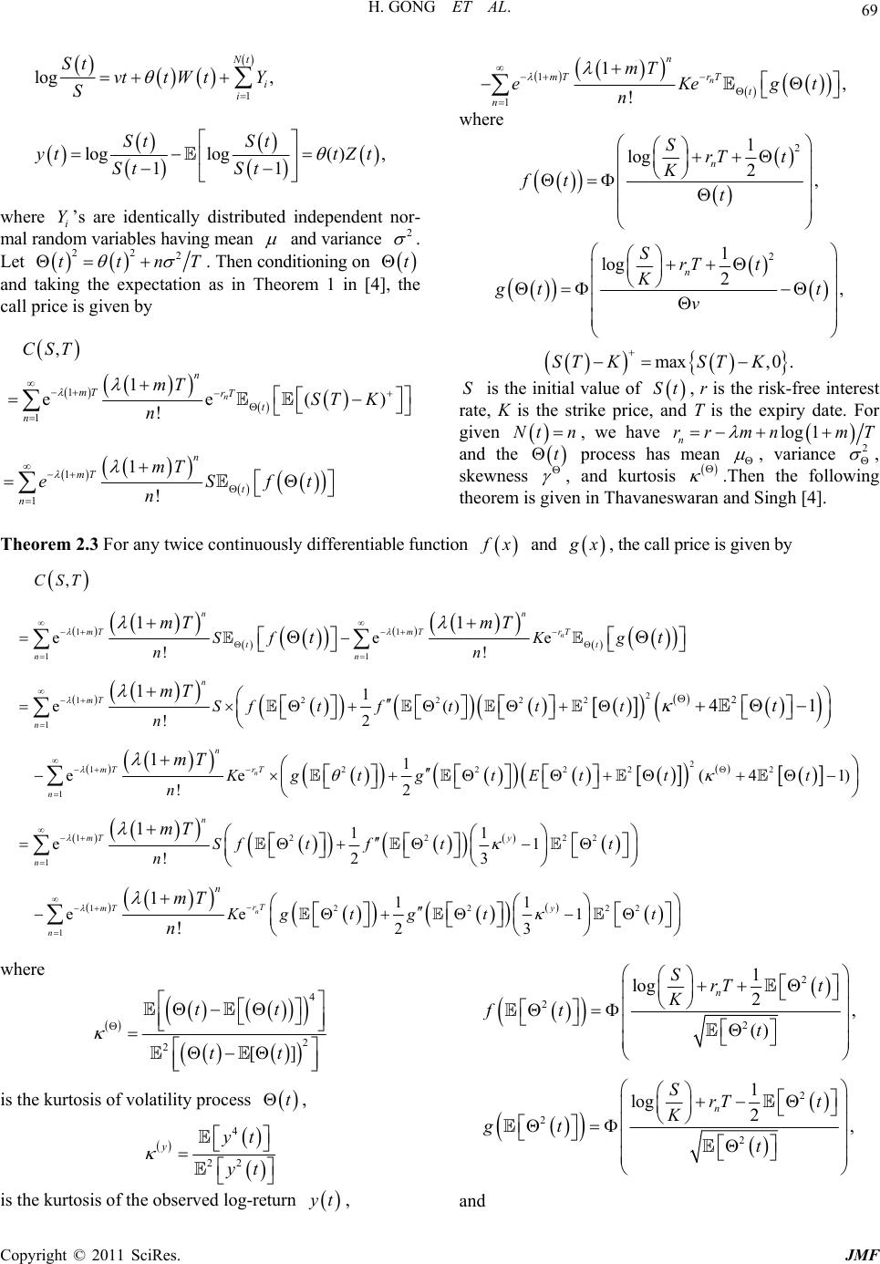

69 H. GONG ET AL.
  

 
   
1
log ,
loglog( ),
11
Nt
i
i
St vttWtY
S
St St
yt tZt
St St



 

 





where ’s are identically distributed independent nor-
mi
Y
al random variables having mean

and variance 2

.
 
Let22
2
ttT  . Then conditioning on n 


t
g the en as in Theoand takxpectatiorem 1 in [4
call price is given by
in], the






1
1
,
1
ee()
!n
n
mT rT t
n
CST
mT ST K
n


 














1
1
1
!
n
mT
t
n
mT
eS
n













 
1
1
1,
!


 





n
n
mT rT t
n
mT
eKeg
n
t
where
 


2 1
log 2,
n
SrT t
K
ft t







 





 
2 1
2,
n
rT t
K
log S
g
tt





 


v





is the initial value of
   
max,0.ST KST K


S


St,
nd r is the risk-free interes K is the strike price, aT is the expiry date. For
n
t
rate,
give


Nt n

, we have


log 1
n
rr mnmT   
and the


t , variance 2


process hasean m


ft
,
skewness


, an
rem is given id kurn thefollo n Thavangh4].
erentiable function
tosis
neswara



n a
.The
nd Si [wing theo
and


g
x Theorem 2.3 For any twice continuously diff


f
x, the call price i s given by






 




 

 


 






 
1 1
1
ee
!
mT mT
t
n n
n
Sf
n
t
   

 








1
2
122
22
1
12
1
2
e
!
1
e()
!2
1
ee
!2
11
141
1
n
n
n
rT
t
mT
n
n
rT mT
n
K g
n
Sft fttt
n
Kg tg
n
mTmT t
mT t
mT






 








 







 


  











  


 
,
n
CST










   





2
222 2
2
2
1
(4 1)
2
1
2
!n
rT y
n
tE ttt
t
Kgt g
T
n





 










 

 


22
2 22
1
1
3
1
1
3
yt
t t
 





 
12
1
1
1
e
!
ee
1
1
n
mT
n
mT
n
Sf t f
n
mT
m



















 

 



here






w

  
  

4
tt


 



2
2[]tt



 



is the kurtosis of volatility process

t,



4
22
yyt
yt










is the kurtosis of the observed log-return

y
t,



2
22
n
K
t









2
1
log
,
()
SrT t
ft
 
 














2
2
2
1
log 2,
n
SrTt
K
gt t

 
 
















and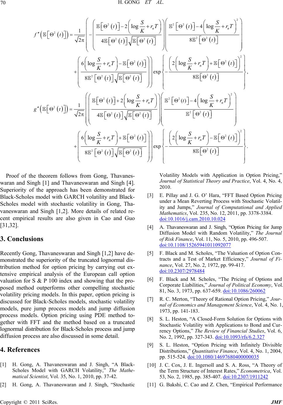

H. GONG ET AL.
70



 



 
2
222
2
22
22
2
22 2
24
1
8
24
2 6
exp
8
log log
log log
nn
n
tt
ft t
tt
t
tt
SS
rT rT
KK
S
SrT K
K
 
  





  
 


 

 
 



 


 
 





 

 
  

 





 













 

2
2
2
2
222
2
22
22
2
,
8
2()4
1
24
6
log log
log
n
nn
n
t
t
tt
gt t
tt
t
rT
SS
rT rT
KK
SrT
K


 
  





 
 




















 
 


 
  
 



 


 





















2
2
2
22 2
2
exp .
8
8
log nt
t
tt
SrT
K





 

 



   





 










 


 



Proof of the theorem follows from Gong, Thavanes-
warand Singh [4].
een donstrated for
Black-Scholes model with GARCH volatility and Black-
Scholes model with stochastic volatility in Gong, Tha-
vaneswaran and Singh [1,2]. More details of related re-
Cao and Guo
[31,32].
3. Conclusions
Recently Gong, Thavaneswaran and Singh [1,2] have de-
monstrated the superiority of the truncated lognormal dis-
tribution method for option pricing by carrying out ex-
tensive empirical analysis of the European call option
valuation for S & P 100 index and showing that the pro-
posed method outperforms other compelling stochastic
volatility pricing models. In this paper, option pricing is
discussed for Black-Scholes models, stochastic volatility
models, pure jump process models and jump diffusion
process models. Option pricing using PDE method to-
gether with FFT and the method based on a truncated
lognormal distribution for Black-Scholes process and jump
diffusion process are also discussed in some detail.
4. References
[1] H. Gong, A. Thavaneswaran and J. Singh, “A Black-
Scholes Model with GARCH Volatility,” The Mathe-
matical Scientist, Vol. 35, No. 1, 2010, pp. 37-42.
[2]
Volatility Models with Application in Option Pricing,”
Journal of Statistical Theory and Practice, Vol. 4, No. 4,
2010.
[3] E. Pillay and J. G. O’ Hara, “FFT Based Option Pricg
under a Mean Reverting Process with Stochastic Volatil-
ity and Jumps,” Journal of Computational and Applied
Mathematics, Vol. 235, No. 12, 2011, pp. 3378-3384.
doi:10.1016/j.cam.2010.10.024
waran and Singh [1] and Thavanesn a
Superiority of the approach has bem
cent empirical results are also given in
H. Gong, A. Thavaneswaran and J. Singh, “Stochastic
in
A. Thavaneswaran and J. Singh, “Option Pricing for Jump
Diffusion Model with Random Volatility,” The Journal
of Risk Finance, Vol. 11, No. 5, 2010, pp. 496-507.
doi:10.1108/15265941011092077
[4]
[5] F. Black and M. Scholes, “The Valuation of Option Con-
tracts and a Test of Market Efficiency,” Journal of Fi-
nance, Vol. 27, No. 2, 1972, pp. 99-417.
doi:10.2307/2978484
[6] F. Black and M. Scholes, “The Pricing of Options and
Corporate Liabilities,” Journal of Political Economy, Vol.
81, No. 3, 1973, pp. 637-659. doi:10.1086/260062
[7] R. C. Merton, “Theory of Rational Option Pricing,” Jour-
nal of Economics and Management Science, Vol. 4, No. 1,
1973, pp. 141-183.
[8] S. L. Heston, “A Closed-Form Solution for Options with
Stochastic Volatility with Applications to Bond and Cur-
rency Options,” The Review of Financial Studies, Vol. 6,
No. 2, 1992, pp. 327-343. doi:10.1093/rfs/6.2.327
[9] S. L. Heston, “Option Pricing with Infinitely Divisible
Distributions,” Quantitative Finance, Vol. 4, No. 1, 2004,
pp. 515-524. doi:10.1080/14697680400000035
[10] J. C. Cox, J. E. Ingersoll and S. A. Ross, “A Theory of
the Term Structure of Interest Rates,” Econometrica, Vol.
53, No. 2, 1985, pp. 385-407. doi:10.2307/1911242
[11] G. Bakshi, C. Cao and Z. Chen, “Empirical Performance

71 H. GONG ET AL.
of Altemative Option Pricing Models,” Journal of Finance,
Vol. 52, No. 5, 1997, pp. 2003-2049.
doi:10.2307/2329472
[12] L. O. Scott, “Option Pricing When the Variance Changes
Randomly: Theory, Estimation, and an Application,” Jour-
nal of Financial and Quantitative Analysis, Vol. 22, No.
4, 1987, pp. 419-438. doi:10.2307/2330793
hite, “The Pricing of Options on Assets
Volatilities,” Journal of Finance, Vol. 42,
No. 2, 1987, pp. 281-300. doi:10.2307/2328253
[13] J. Hull and A. W
with Stochastic
[14] J. Hull and A. White, “An Analysis of the Bias in Option
Pricing Caused by a Stochastic Volatility,” Journal of In-
ternational Economics, Vol. 24, No. 4, 1988, pp. 129-
145.
[15] P. Ritchken and R. Trevor, “Pricing Options under Gen-
eralized GARCH and Stochastic Volatility Processes,”
Journal of Finance, Vol. 59, No. 1, 1999, pp. 377-402.
doi:10.1111/0022-1082.00109
[16] J. B. Wiggins, “Option Values under Stochastic Volatil-
ities,” Journal of Financial Economics, Vol. 19, 1987, pp.
351-372. doi:10.1016/0304-405X(87)90009-2
[17] S. L. Heston and S. Nandi, “A Closed-Form GARCH
Option Valuation Model,” The Review of Financial
ies, Vol. 13, No. 1, 2000, pp. 585-625. Stud-
s/13.3.585doi:10.1093/rf
. K. Siu and L. Chan, “Option Pricing[18] R. J. Elliot, T for
GARCH Models with Markov Switching,” International
Journal of Theoretical and Applied Finance, Vol. 9, No.
6, 2006, pp. 825-841. doi:10.1142/S0219024906003846
[19] P. Christoffersen, S. Heston and K. Jacobs, “Option Val-
uation with Conditional Skewness,” Journal of Eco- no-
mtrics, Vol. 131, No. 1-2, 2006, pp. 253-284.
[20] L. Mercuri, “Option Pricing in a GARCH Model with
Tempered Stable Innovations,” Finance Research Letter,
Vol. 5, No. 3, 2008, pp. 172-182.
doi:10.1016/j.frl.2008.05.003
[21] A. M. Badescu and R. J. Kulperger, “GARCH Optio
Oricing: a Semiparametric ApprInsurance Mathe-
n
oach,”
matics and Economics, Vol. 43, No. 1, 2008, pp. 69-84.
doi:10.1016/j.insmatheco.2007.09.011
[22] G. Barone-Adesi, H. Rasmussen and C. Ravanelli, “An
Option Pricing Formula for the GARCH Diffusion Model,”
Computational Statistics and Data Analysis, Vol. 49, No.
2, 2005, pp. 287-310. doi:10.1016/j.csda.2004.05.014
[23] G. Barone-Adesi, R. F. Engle and L. Mancini, “A
GARCH Option Pricing Model with Filtered Historical
Simulation,” Review of Financial Studies, Vol. 21, No. 3,
2008, pp. 1223-1258. doi:10.1093/rfs/hhn031
[24] A. Thavaneswaran, S. Peiris and J. Sin
Kurtosis and Option Pgh, “Derivation of ricing Formulas for Popular Vola-
tility Mode ls with Applications in Fina nce,” Communica-
tions in Statistics.Theory and Methods, Vol. 37, 2008, pp.
1799-1814. doi:10.1080/03610920701826435
[25] A. Thavaneswaran, J. Singh and S. S. Appadoo, “Option
Pricing for Some Stochastic Volatility Models,” Journal
of Risk Finance, Vol. 7, No. 4, 2006, pp. 425-445.
doi:10.1108/15265940610688982
[26] S. J. Taylor, “Asset Price Dynamics, Volatility, and Pre-
diction,” Princeton University Press, Princeton, 2005.
[27] J. M. Steele, “Stochastic Calculus and Financial Applica-
tions,” Springer, New York, 2001.
tility,” European Journal
[28] J. Vecer, “Stochastic Finance: A Numeraire Approach,”
Chapman & Hall/CRC Press, London, 2011.
[29] H. Y. Wong and Y. W. Lo, “Option Pricing with Mean
Reversion and Stochastic Vola
of Operational Research, Vol. 197, No. 1, 2009, pp. 179-
187. doi:10.1016/j.ejor.2008.05.014
[30] D. Duffie, J. Pan and K. Singleton, “Transform Analysis
and Asset Pricing for Affine Jump-Diffusion,” Econo-
metrica, Vol. 68, No. 6, 2000, pp. 1343-1376.
doi:10.1111/1468-0262.00164
[31] L. Cao and Z. F. Guo, “Applying Gradient Estimation
Financial
Technique to Estimate Gradients of European Call fol-
lowing Variance-Gamma,” Proceedings of Global Con-
ference on Business and Finance, Vol. 6, No. 2, 2011, pp.
12-18.
[32] L. Cao and Z. F. Guo, “Applying Variance Gamma Cor-
related to Estimate Optimal Portfolio of Variance Swap,”
Proceedings of International Conference of
Engineering, London, 6-8 July 2011.