Engineering, 2009, 1, 133-139
doi:10.4236/eng.2009.13016 Published Online November 2009 (http://www.scirp.org/journal/eng).
Effect of Oscillating Jet Velocity on the Jet Impingement
Cooling of an Isothermal Surface
Nawaf H. SAEID
Department of Mechanical, Manufacturing and Materials Engineering,
The University of Nottingham Malaysia Campus, Semenyih, Malaysia
Received January 10, 2009; revised February 21, 2009; accepted February 23, 2009
Abstract
Numerical investigation of the unsteady two-dimensional slot jet impingement cooling of a horizontal heat
source is carried out in the present article. The jet velocity is assumed to be in the laminar flow regime and it
has a periodic variation with the flow time. The solution is started with zero initial velocity components and
constant initial temperature, which is same as the jet temperature. After few periods of oscillation the flow
and heat transfer process become periodic. The performance of the jet impingement cooling is evaluated by
calculation of friction coefficient and Nusselt number. Parametric study is carried out and the results are
presented to show the effects of the periodic jet velocity on the heat and fluid flow. The results indicate that
the average Nusselt number and the average friction coefficient are oscillating following the jet velocity os-
cillation with a small phase shift at small periods. The simulation results show that the combination of Re
=200 with the period of the jet velocity between 1.5 sec and 2.0 sec and high amplitude (0.25 m/s to 0.3 m/s)
gives average friction coefficient and Nusselt number higher than the respective steady-state values.
Keywords: Heat Transfer, Unsteady Convection, Jet Impingement, Periodic Oscillation, Numerical Study
1. Introduction
Jet Impinging is widely used for cooling, heating and
drying in several industrial applications due to their high
heat removal rates with relatively low pressure drop. In
many industrial applications, such as in cooling of elec-
tronics surfaces, the jet outflow is confined between the
heated surface and an opposing surface in which the jet
orifice is located. Recently many researchers [1–7] have
carried out numerical and experimental investigations of
laminar impinging jet cooling with different fluids and
under various boundary conditions.
The literature review reveals that the behavior of the
two-dimensional laminar impinging jet is not well un-
derstood. Numerical results of Li et al. [8] indicate that
there exist two different solutions in some range of geo-
metric and flow parameters of the laminar jet impinge-
ment flow. The two steady flow patterns are obtained
under identical boundary conditions but only with dif-
ferent initial flow fields. This indicates that the unsteady
state analysis is important to have better understanding
of the flow and heat transfer in jet impingement. Fi-
nite-difference approach was used by Chiriac and Ortega
[9] in computing the steady and unsteady flow and heat
transfer due to a confined two-dimensional slot jet im-
pinging on an isothermal plate. The jet Reynolds number
was varied from Re=250 to 750 for a Prandtl number of
0.7 and a fixed jet-to-plate spacing of H=W= 5. They
found that the flow becomes unsteady at a Reynolds
number between 585 and 610. Chung et al. [10] have
solved the unsteady compressible Navier–Stokes equa-
tions for impinging jet flow using a high-order finite dif-
ference method with non-reflecting boundary conditions.
Their results show that the impingement heat transfer is
very unsteady and the unsteadiness is caused by the pri-
mary vortices emanating from the jet nozzle.
Camci and Herr [11] have showed that it is possible to
convert a stationary impinging cooling jet into a self-
oscillating-impinging jet by adding two communication
ports at the throat section. Their experimental results
show that a self-oscillating turbulent impinging-jet con-
figuration is extremely beneficial in enhancing the heat
removal performance of a conventional (stationary) im-
pinging jet. It is of great importance to investigate the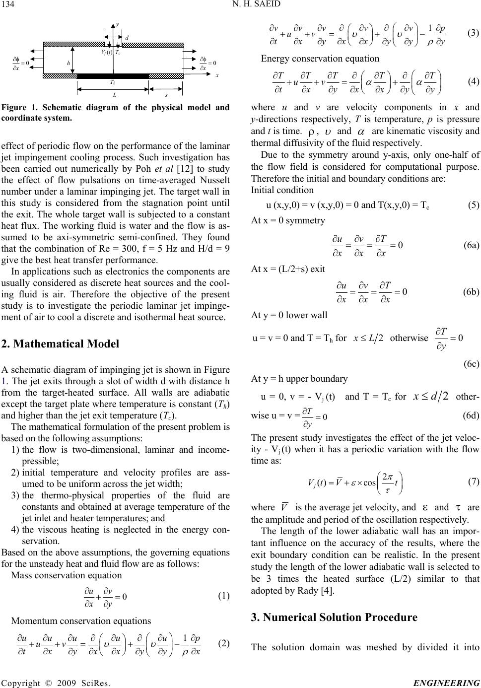

N. H. SAEID 134
y
d
Vj (t) Tc
0


x h 0 

x
x
Th
L s
Figure 1. Schematic diagram of the physical model and
coordinate system.
effect of periodic flow on the performance of the laminar
jet impingement cooling process. Such investigation has
been carried out numerically by Poh et al [12] to study
the effect of flow pulsations on time-averaged Nusselt
number under a laminar impinging jet. The target wall in
this study is considered from the stagnation point until
the exit. The whole target wall is subjected to a constant
heat flux. The working fluid is water and the flow is as-
sumed to be axi-symmetric semi-confined. They found
that the combination of Re = 300, f = 5 Hz and H/d = 9
give the best heat transfer performance.
In applications such as electronics the components are
usually considered as discrete heat sources and the cool-
ing fluid is air. Therefore the objective of the present
study is to investigate the periodic laminar jet impinge-
ment of air to cool a discrete and isothermal heat source.
2. Mathematical Model
A schematic diagram of impinging jet is shown in Figure
1. The jet exits through a slot of width d with distance h
from the target-heated surface. All walls are adiabatic
except the target plate where temperature is constant (Th)
and higher than the jet exit temperature (Tc).
The mathematical formulation of the present problem is
based on the following assumptions:
1) the flow is two-dimensional, laminar and income-
pressible;
2) initial temperature and velocity profiles are ass-
umed to be uniform across the jet width;
3) the thermo-physical properties of the fluid are
constants and obtained at average temperature of the
jet inlet and heater temperatures; and
4) the viscous heating is neglected in the energy con-
servation.
Based on the above assumptions, the governing equations
for the unsteady heat and fluid flow are as follows:
Mass conservation equation
0
uv
xy


 (1)
Momentum conservation equations
1uuu uu
uv
txyxxyy


  

 
 
 

1vvvvv
uv
txyxxyy


 p
y

 


 

 
 (3)
Energy conservation equation
TTTTT
uv
txyxxyy





 
  




(4)
where u and v are velocity components in x and
y-directions respectively, T is temperature, p is pressure
and t is time.

,

and

are kinematic viscosity and
thermal diffusivity of the fluid respectively.
Due to the symmetry around y-axis, only one-half of
the flow field is considered for computational purpose.
Therefore the initial and boundary conditions are:
Initial condition
u (x,y,0) = v (x,y,0) = 0 and T(x,y,0) = Tc (5)
At x = 0 symmetry
0
uvT
xxx



 (6a)
At x = (L/2+s) exit
0
uvT
xxx



 (6b)
At y = 0 lower wall
u = v = 0 and T = Th for 2
x
L

otherwise 0
T
y



(6c)
At y = h upper boundary
u = 0, v = - Vj (t) and T = Tc for 2dx  other-
wise u = v =0
T
y


 (6d)
The present study investigates the effect of the jet veloc-
ity - Vj (t) when it has a periodic variation with the flow
time as:
2
() cos
j
Vt Vt



 



(7)
where V is the average jet velocity, and and 

are
the amplitude and period of the oscillation respectively.
The length of the lower adiabatic wall has an impor-
tant influence on the accuracy of the results, where the
exit boundary condition can be realistic. In the present
study the length of the lower adiabatic wall is selected to
be 3 times the heated surface (L/2) similar to that
adopted by Rady [4].
3. Numerical Solution Procedure
p
x
(2) The solution domain was meshed by divided it into

N. H. SAEID135
spacing quadrilateral cells. The cells were clusters near
the symmetry axis where steep variations in velocity and
temperature are expected.
FLUENT 6.3 is used as a tool for numerical solution
of the governing equations based on finite-volume me-
thod. QUICK discretization scheme [13] is selected for
convection-diffusion formulation for momentum and
energy equations. The central differencing scheme is
used for the diffusion terms. The discretized equations
were solved following the SIMPLEC algorithm [14].
Relaxation factors are used to avoid divergence in the
iteration. The typical relaxation factors were used as 0.7
for momentum equations, 0.3 for the pressure and 1.0 for
the energy equation. For time integral the first order im-
plicit scheme is used, which is unconditional stable.
The convergence criterion is based on the residual in
the governing equations. The maximum residual in the
energy was 10-7 and the residual of other variables were
lower than 10-5 in the converged solution. In all the
computational cases the global heat and mass balance are
satisfied in the converged solution within 10-3 %. 
Air is used as working fluid with constant physical
properties. Most of the benchmark results are presented
with constant Prandtl number, Pr = 0.71, for air. The
average temperature between the cold incoming jet and
the hot plate is selected to be 300K so that the Prandtl
number is approximately 0.71. The plate temperature is
fixed at 310K and the incoming jet temperature is main-
tained at 290K. The properties were found from the
properties tables of air at an average temperature of
300K as: density

= 1.1614 kg/m3, specific heat cp =
1007 J/kgK, thermal conductivity k = 0.0263 W/mK and
viscosity of

= 1.84610-5 kg/ms.
4. Results and Discussions
The performance of the jet impingement cooling is
evaluated based on the friction coefficient and Nusselt
number, which are defined respectively as:

2
1
2 20
1
2
w
fy
cuy
V



 V  (8)
 
0
w
hc
y
hc
qd
NudT yTT
TTk 

 (9)
where is the wall shear stress and qw is the wall
heat flux. The average friction coefficient and the aver-
age Nusselt number at the heated plate are also calcu-
lated by integrating the local values over the length of
the plate as follows:
w

2
0
2L
ff
cc
L

0
1
2
3
4
5
6
7
8
00.02 0.04 0.06 0.080.1
Present using (50  25) mesh
Present using (100  50) mesh
Nu Present using (200  100) mesh
■ Radi (2000)
▲ Al Sanea (1992)
x (m)
(a)
0
1
2
3
4
5
6
7
8
9
00.02 0.040.06 0.080.1
Present using (50  25) mesh
Present using (100
 50) mesh
f
c
2
10 Present using (200  100) mesh
▲ Al Sanea (1992)
x (m)
(b)
Figure 2. (a) Variation of Nusselt number along the heated
plate.Re = 200, h/d = 4, L/d = 20 and Pr = 0.71; (b) Variation
of friction coefficient along the heated plate.Re = 200, h/d = 4,
L/d = 20 and Pr = 0.71.
Table 1. Values of Nu with grid refinement compared
with reference values.
Nu
Present results using different mesh
sizes
Re Al-Senea
(1992)
Rady
(2000)
(50 25) (10050) (200

100)
1001.596 1.46 1.4880 1.4743 1.4599
2002.505 2.38 2.4332 2.4539 2.4473
Table 2. Values of average friction coefficient with grid
refinement.
f
c
Present results using different mesh sizes
Re V
(m/s)
(50

25) (10050) (200

100)
1000.1590.030436 0.031934 0.031900
2000.3180.025352 0.028638 0.029346
2
0
2L
NuNu dx
L
 (11)
dx
(10)

N. H. SAEID 136
The effect of mesh size on the accuracy of calculating
friction coefficient and Nusselt number is studied for
steady flow with constant jet velocity. The present results
obtained using different mesh sizes are compared with
the results of Al-Senea [2] and Rady [4]. The results
presented in Figure 2(a) and Table 1 shows the compari-
son of local and average Nusselt number respectively.
Figure 2(b) and Table 2 show the simulation results for
local and average friction coefficient respectively. The
present results show that the mesh with 10050 quadri-
lateral cells in the x and y directions respectively gives
results with acceptable accuracy. The mesh is designed
so that the jet width, which is d/2 = 0.005 m is divided
into 10 cells (control volumes). The heated surface L/2 =
0.1 m (which gives L/d = 20) is discretized into 50 divi-
sions and the remaining adiabatic lower wall is divided
into 50 divisions. The height h = 0.04 m (where h/d = 4)
in the vertical direction is divided into 50 divisions. The
results shown in Figures 2 and Tables 1 and 2 also show
that halving or duplicating the mesh size have minor ef-
fects on the values of the Nusselt number and friction
coefficient. Therefore the results obtained using mesh
with 10050 quadrilateral cells can be considered as
grid independent results. Good agreements of the present
results with those references cited in [2] and [4] are ob-
served for two different values of the Reynolds number
in the laminar regime. Where Re is the Reynolds number
defined based on average jet velocity and jet width as:

 dVRe . It is worth mentioning that the values of
f
c are not listed in the references [2] and [4].
In unsteady flows in general and especially periodic
flows, the time step size has a great influence of the ac-
curacy of the results. The time step size can be made to
be a function of the frequency/period of the flow oscilla-
tion as implemented by Saeid [15,16]. In the present pe-
riodic flow problem, the time step size is selected a func-
tion of the period of the jet flow oscillation as
100t sec.
To study the effect of the amplitude of the
oscillation on the flow, the jet velocity is made to osci-
llate with time according to Equation (7) with fixed
values of period


= 10 sec and Re = 200. It is
important to note that the definition of Reynolds number
in the present study is based on average jet velocity. To
get Re = 200, the average jet velocity should be 0.318
m/s since the geometry of the problem and the air
properties are assumed constants. Therefore the maxi-
mum amplitude of the oscillation is selected to be 0.3
m/s so that there will be always positive impinging
velocity on the target surface.
The initial conditions in the unsteady simulation are
defined in (5) which assume that the solution domain is
filled with stagnant air at jet temperature. Then the jet
starts to inflow and the target surface temperature in-
0.5
1
1.5
2
2.5
3
3.5
8082.5 8587.5 9092.5 9597.5100

= 0.0, 0.1, 0.15, 0.2, 0.25, 0.3 m/s
Nu
t (sec)
(a)
(b)
Figure 3. (a) Oscillation of
N
u with = 10 sec and Re =
200; (b) Oscillation of

f
c with = 10 sec and Re = 200. 
creases suddenly from Tc to Th. At this time the value of
Nusselt number goes to very high value. Then, when the
jet velocity oscillates the calculated values of average
Nusselt number is found to oscillate accordingly. This
oscillation becomes steady periodic oscillation after
some periods of oscillation. The steady periodic oscilla-
tion is achieved when the amplitude and the average
values of the average Nusselt number become constant
for different periods.
The numerical results of oscillation of the average
Nusselt number in the ninth and tenth periods with

= 10
sec and Re = 200 is shown in Figure 3(a). The corre-
sponding oscillation of the average friction coefficient in
the ninth and tenth periods is shown in Figure 3(b).
Both the Nusselt number and the friction coefficient
are observed to oscillate in all the cases for different
values of

with a small phase change with the jet
oscillation (which is cosine wave). For small values of
the amplitude of the jet inflow oscillation ( = 0.1 m/s
to 0.2 m/s), the calculated average Nusselt number is
oscillating in smooth sinusoidal oscillation as shown in
Figure 3.

The effect of the period of the jet inflow velocity is
studied and the results are shown in Figures 4a and 4b as
Nu against ωt and f c against ωt respectively, where ω
is the frequency of the oscillation ( 2). Figure 4
shows clearly how the period of the jet velocity
influences the periodic variation of Nu and f c for

N. H. SAEID 137
1.75
2
2.25
2.5
2.75
3
56.832 57.83258.832 59.832 60.83261.832 62.832
Nu

= 1, 1.5, 2, 3, 5, 10 sec
ωt
1o
o
t
t
NuNu dt



 (13)
where to represents the time required to reach the steady
periodic oscillation process (around 9 periods of oscilla-
tion). Figures 5(a) and 5(b) show respectively the varia-
tion of Nu and f c with for different values of the
period of the jet oscillation and constant Re =200.

For small values of

(less than 0.15 m/s), the cyclic
average value of the space-averaged Nusselt number (Nu)
is decreasing with the increase of either or 

as
shown in Figure 5(a). Figure 5(b) shows that f
c also
decr- eases with the increase of either or for small
values of
 

.
(a)
0.015
0.02
0.025
0.03
0.035
0.04
0.045
56.832 57.832 58.832 59.832 60.832 61.832 62.832
f
c

= 1, 1.5, 2, 3, 5, 10 sec
ωt
This means that the cooling process is deteriorated by
using oscillating jet under these conditions. The results
presented in Figure 5 show also the possibility of cooling
enhancement when the period of the jet velocity between
1.5 sec and 2.0 sec and high amplitude (0.25 m/s to 0.3
m/s) with Re = 200.
At these conditions the cyclic average value of both the
space-averaged friction coefficient and Nusselt number are
found to be higher than the steady-state value (when

=
0) as shown in Figure 5.
(b)
Figure 4. (a) Periodic oscillation of Nu with = 0.1 m/s,
and Re = 200; (b) Periodic oscillation of f
c with

= 0.1
m/s, and Re = 200.
Re = 200 with forcing amplitude = 0.1. At high
values of


there will be enough time for the
momentum and heat transfer to follow the effect of the
periodic variation of the jet velocity. Therefore the avera-
ge Nusselt number and average friction coefficient are
found to follow the jet velocity function (cosine-
function) for high values of

(5 and 10) as shown in
Figure 4.
2.2
2.3
2.4
2.5
2.6
00.05 0.10.150.20.25 0.3
τ = 1.0 sec τ = 1.5 sec τ = 2.0 sec
τ = 3.0 sec τ = 5.0 sec τ = 10 sec
Nu

(m/s)
(a)
The amplitude of both the average Nusselt number and
average friction coefficient oscillation is higher for larger
periods of jet oscillation. Figure 4 shows also, as

decreases, the peak values of average Nusselt number
and average friction coefficient are delayed.
The results presented in Figures 3 and 4 show the
oscillation of both the average Nusselt number and
average friction coefficient according to the jet velocity
oscillation; therefore it is important to introduce the
cyclic average value of the space-averaged friction
coefficient and Nusselt number defined respectively as:
0.025
0.026
0.027
0.028
0.029
0.03
0.031
0.032
00.05 0.1 0.15 0.20.25 0.3
τ = 1.0 sec τ = 1.5 sec τ = 2.0 sec
τ = 3.0 sec τ = 5.0 sec τ = 10 sec
f
c

(
m/s
)
(b)
Figure 5. (a) Variation of Nu with at Re =200; (b)
Variation of

f
c with
1o
o
t
ff
t
cc



dt (12)

at Re =200.

N. H. SAEID 138
Figure 6. Isotherms,
T
= 1K (left) and streamlines (right) for a cycle of oscillation with ε = 0.3 m/s, = 2 sec, and Re= 200. 
0
0.5
1
1.5
2
2.5
3
3.5
4
99.1 9.29.3 9.4 9.5 9.6 9.79.8 9.910
Re = 100, 200, 300
Nu
t (sec )
(a)
0
0.01
0.02
0.03
0.04
0.05
99.1 9.2 9.3 9.4 9.5 9.6 9.7 9.8 9.910
Re = 300, 200, 100
f
c
t (s e c)
(b)
Figure 7. (a) Periodic oscillation of Nu with = 0.1 m/s
and = 1 sec; (b) Periodic oscillation of

f
c with

= 0.1
m/s and = 1 sec.

From the results presented in Figure 5 it can be seen that
the increase of Nu is about 2.3% while the increase in
f
c is 2.6% when the period of the jet velocity is 2.0 sec
and amplitude of 0.3 m/s with Re = 200.
In order to have better understanding, the period of the
last cycle is divided into eight time steps. At each time
step the isotherms and streamlines are shown in Figure 6
for the periodic oscillation with = 0.3 m/s,


= 2 sec
and Re = 200.
The isotherms show some high temperature points on
the heated target wall. These hot spots are moving along
the heated surface according to the jet velocity oscillation.
Obviously when the jet velocity is small near the
minimum at t = 84 sec (=0.018 m/s) the
temperature near the target surface is high. Figure 6
show that the oscillation of the jet velocity leads to wash
away the heated spots after they appear above the heated
surface with some delay. The average Nusselt number
j
V
value at t = 8

sec (= 0.530 m/s) is higher that that
j
V
at maximum velocity at t = 88 sec, (= 0.618 m/s).
j
V
Finally the effect of the Reynolds number on the peri-
odic jet impingement cooling process is studied and the
results are depicted on Figure 7. The range of the Rey-
nolds number is selected to be in the laminar regime. Ob-
viously increasing the Reynolds number by increasing the
jet velocity leads to the increase in the average Nusselt
number and reduce the friction coefficient as shown in
Figure 7(a) and (b) respectively. It is observed that the
oscillation of both the average Nusselt number and the av-

N. H. SAEID139
erage friction coefficient at different values of Re have
small phase shift in the steady periodic oscillation as
shown in Figure 7.
5. Conclusions
In the present study the periodic laminar jet impingement
cooling of a horizontal surface is consider for numerical
investigation. The periodic jet impingement cooling is
generated when there is periodic oscillation of the jet
inflow velocity. It has been shown that the Nusselt num-
ber oscillates as a result of oscillating jet inflow velocity.
The results are presented to show the effects of the am-
plitude and the period of the jet velocity on the Nusselt
number and friction coefficient in the steady periodic
state. The results indicate that both the average friction
coefficient and Nusselt number are oscillating following
the jet velocity oscillation with a small phase change.
The periodic average friction coefficient and the Nusselt
number are found to follow the jet velocity function for
high values of period

. This is due to the fact that
there is enough time for the momentum and heat transfer
to follow the effect of the periodic variation of the jet
velocity. The simulation results show that it is possible to
enhance the cooling process for some combination of the
Reynolds number with period and amplitude of the jet
velocity. The combination of Re =200 with the period
of the jet velocity between 1.5 sec and 2.0 sec and high
amplitude (0.25 m/s to 0.3 m/s) gives average friction co-
efficient and Nusselt number higher than the respective
steady-state values.
6. References
[1] E. M. Sparrow and T. C. Wong, “Impingement transfer
coefficient due to initially laminar slot jets,” Int. J. Heat
Mass Transfer, Vol. 18, pp. 597–605, 1975.
[2] S. Al-Sanea, “A numerical study of the flow and heat
transfer characteristics of an impinging laminar slot-jet
including crossflow effects,” Int. J. Heat Mass Transfer,
Vol. 35, pp. 2501–2513, 1992
[3] Z. H. Lin, Y. J. Chou, and Y. H. Hung, “Heat transfer
behaviors of a confined slot jet impingement,” Int. J. Heat
Mass Transfer, Vol. 40, pp. 1095–1107, 1997.
[4] M. A. Rady, “Buoyancy effects on the flow and heat
transfer characteristics of an impinging semi-confined
laminar slot jet,” Int. J. Trans. Phenomena, Vol. 2, pp.
113–126, 2000.
[5] H. Chattopadhyay and S. K. Saha, “Simulation of laminar
slot jets impinging on a moving surface,” J. Heat Transfer,
Vol. 124, pp. 1049-1055, 2002.
[6] L. B. Y. Aldabbagh, I. Sezai, and A. A. Mohamad,
“Three- dimensional investigation of a laminar impinging
square jet interaction with cross flow,” J. Heat Transfer,
Vol. 125, pp. 243–249, 2003.
[7] D. Sahoo and M. A. R. Sharif, “Numerical modeling of
slot-jet impingement cooling of a constant heat flux sur-
face confined by a parallel wall,” Int. J. Therm. Sci., Vol.
43, pp. 877–887, 2004.
[8] X. Li, J. L. Gaddis, and T. Wang, “Multiple flow patterns
and heat transfer in confined jet impingement,” Int. J.
Heat Fluid Flow, Vol. 26, pp. 746–754, 2005.
[9] V. A. Chiriac and A. Ortega, “A numerical study of the
unsteady flow and heat transfer in a transitional confined
slot jet impinging on an isothermal surface,” Int. J. Heat
Mass Transfer, Vol. 45, pp. 1237–1248, 2002.
[10] Y. M. Chung, K. H. Lao, and N. D. Sandham, “Numeri-
cal study of momentum and heat transfer in unsteady im-
pinging jets,” Int. J. Heat Fluid Flow, Vol. 23, pp.
592–600, 2002.
[11] C. Camci and F. Herr, “Forced convection heat transfer
enhancement using a self-oscillating impinging planar
jet,” J. Heat Transfer, Vol. 124, pp. 770–782, 2002.
[12] H. J. Poh, K. Kumar, and A. S. Mujumdar, “Heat transfer
from a pulsed laminar impinging jet,” Int. Comm. Heat
Mass Transfer, Vol. 32, pp. 1317–1324, 2005.T. Hayase,
J. A. C. Humphrey, and R. Greif, “A consistently formu-
lated QUICK scheme for fast and stable convergence using
finite-volume iterative calculation procedures,” J. Comput.
Phys., Vol. 98, pp. 108–118, 1992.
[14] H. K. Versteeg and W. Malalasekera, “Computational
fluid dynamics: An introduction,” Longman, 1995.
[15] N. H. Saeid, “Periodic free convection from vertical plate
subjected to periodic surface temperature oscillation,” Int.
J. Therm. Sci., Vol. 43, pp. 569–574, 2004.
[16] N. H. Saeid, “Mixed convection flow along a vertical
plate subjected to time-periodic surface temperature os-
cillations,” Int. J. Therm. Sci., Vol. 44, pp. 531–539,
2005.