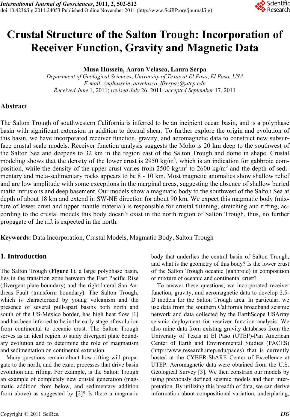
International Journal of Geosciences, 2011, 2, 502-512
doi:10.4236/ijg.2011.24053 Published Online November 2011 (http://www.SciRP.org/journal/ijg)
Crustal Structure of the Salton Trough: Incorporation of
Receiver Function, Gravity and Magnetic Data
Musa Hussein, Aaron Velasco, Laura Serpa
Department of Geological Sci ences, University of Texas at El Paso, El Paso, USA
Received June 1, 2011; revised July 26, 2011; accepted September 17, 2011
Abstract
The Salton Trough of southwestern California is inferred to be an incipient ocean basin, and is a polyphase
basin with significant extension in addition to dextral shear. To further explore the origin and evolution of
this basin, we have incorporated receiver function, gravity, and aeromagnetic data to construct new subsur-
face crustal scale models. Receiver function analysis suggests the Moho is 20 km deep to the southwest of
the Salton Sea and deepens to 32 km in the region east of the Salton Trough and dome in shape. Crustal
modeling shows that the density of the lower crust is 2950 kg/m3, which is an indication for gabbroic com-
position, while the density of the upper crust varies from 2500 kg/m3 to 2600 kg/m3 and the depth of sedi-
mentary and meta-sedimentary rocks appears to be 8 - 10 km. Most magnetic anomalies show shallow relief
and are low amplitude with some exceptions in the marginal areas, suggesting the absence of shallow buried
mafic intrusions and deep basement. Our models show a magmatic body to the southwest of the Salton Sea at
depth of about 18 km and extend in SW-NE direction for about 90 km, We expect this magmatic body (mix-
ture of lower crust and upper mantle material) is responsible for crustal thinning, stretching and rifting, ac-
cording to the crustal models this body doesn’t exist in the north region of Salton Trough, thus, no further
propagate of the rift is expected in the north.
Keywords: Data Incorporation, Crustal Models, Magmatic Body, Salton Trough
1. Introduction
The Salton Trough (Figure 1), a large polyphase basin,
lies in the transition zone between the East Pacific Rise
(divergent plate boundary) and the right-lateral San An-
dreas Fault (transform boundary). The Salton Trough,
which is characterized by young volcanism and the
presence of several pull-apart basins both north and
south of the US-Mexico border, has high heat flow [1]
and has been inferred to be in the early stage of evolution
from continental to oceanic crust. The Salton Trough
serves as an ideal region to study divergent plate bound-
ary evolution and to determine the role of magmatism
and sedimentation on continental extension.
Many questions remain about how rifting will propa-
gate to the north, and the exact processes that drive basin
evolution and rifting. For example, is the Salton Trough
an example of completely new crustal generation (mag-
matic addition from below, and sedimentary addition
from above) as suggested by [2]? Is there a magmatic
body that underlies the central basin of Salton Trough,
and what is the geometry of this body? Is the lower crust
of the Salton Trough oceanic (gabbroic) in composition
or mixture of oceanic and continental crust?
To answer these questions, we incorporated receiver
function, gravity, and aeromagnetic data to develop 2.5-
D models for the Salton Trough area. In particular, we
use data from the southern California broadband seismic
network and data collected by the EarthScope USArray
seismic deployment for receiver function analysis. We
also mine data from existing gravity databases from the
University of Texas at El Paso (UTEP)-Pan American
Center of Earth and Environmental Studies (PACES)
(http://www.research.utep.edu/paces) that is currently
hosted at the CYBER-ShARE Center of Excellence at
UTEP. Aeromagnetic data were obtained from the U.S.
Geological Survey [3]. We then constrain our models by
using previously defined seismic models and their inter-
pretation. By utilizing this breadth of data, we can derive
information about compositional variation, underplating,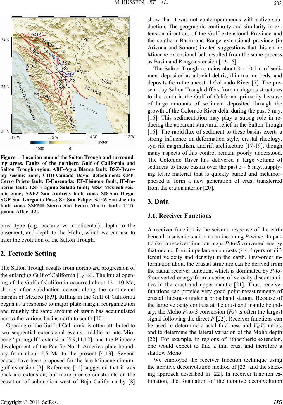

503 M. HUSSEIN ET AL.
Figure 1. Location map of the Salton Trough and surround-
ing areas. Faults of the northern Gulf of California and
Salton Trough region. ABF-Agua Blanca fault; BSZ-Braw-
ley seismic zone; CDD-Canada David detachment; CPF-
Cerro Prieto fault; E-Ensenada; EF-Elsinore fault; IF-Im-
perial fault; LSF-Laguna Salada fault; MSZ-Mexicali seis-
mic zone; SAFZ-San Andreas fault zone; SD-San Diego;
SGP-San Gorgonio Pass; SF-San Felipe; SJFZ-San Jacinto
fault zone; SSPMF-Sierra San Pedro Martir fault; T-Ti-
juana. After [42].
crust type (e.g. oceanic vs. continental), depth to the
basement, and depth to the Moho, which we can use to
infer the evolution of the Salton Trough.
2. Tectonic Setting
The Salton Trough r esu lts f rom no rthw ard pr og ression of
the enlarging Gulf of California [1 ,4-8]. The initial o pen-
ing of the Gulf of California occurred about 12 - 10 Ma,
shortly after subduction ceased along the continental
margin of Mexico [8,9 ]. Rifting in the Gulf of California
began as a response to major plate-margin reorganization
and roughly the same amount of strain has accumulated
across the various basins north to south [10].
Opening of the Gulf of California is often attributed to
two sequential extensional events: middle to late Mio-
cene “protogulf” extension [5,9,11,12], and the Pliocene
development of the Pacific-North America plate bound-
ary from about 5.5 Ma to the present [4,13]. Several
causes have been proposed for the late Miocene circum-
gulf extension [9]. Reference [11] suggested that it was
back arc extension, but more precise constraints on the
cessation of subduction west of Baja California by [8]
show that it was not contemporaneous with active sub-
duction. The geographic continuity and similarity in ex-
tension direction, of the Gulf extensional Province and
the southern Basin and Range extensional province (in
Arizona and Sonora) invited suggestions that this entire
Miocene extension al belt resulted from the same process
as Basin and Range extension [13-15].
The Salton Trough contains about 8 - 10 km of sedi-
ment deposited as alluvial debris, thin marine beds, and
deposits from the ancestral Colorado River [7]. The pre-
sent day Salton Trough differs from analogou s structures
to the south in the Gulf of California primarily because
of large amounts of sediment deposited through the
growth of the Colorado River delta during the past 5 m.y.
[16]. This sedimentation may play a strong role in re-
ducing the apparen t structural relief in the Salton Trough
[16]. The rapid flux of sediment to these basins exerts a
strong influence on deformation style, crustal rheology,
syn-rift magmatism, and rift architecture [17-19], though
many aspects of this control remain poorly understood.
The Colorado River has delivered a large volume of
sediment to these basins over the past 5 - 6 m.y., supply-
ing felsic material that is quickly buried and metamor-
phosed to form a new generation of crust transferred
from the craton interior [20].
3. Data
3.1. Receiver Functions
A receiver function is the seismic response of the earth
beneath a seismic station to an incoming P-wave. In par-
ticular, a receiver function maps P-to-S converted energy
that occurs from impedance contrasts (i.e., layers of dif-
ferent velocity and density) in the earth. First-order in-
formation about the crustal structure can be derived from
the radial receiver function, which is dominated by P-to-
S converted energy from a series of velocity discontinui-
ties in the crust and upper mantle [21]. Thus, receiver
functions can provide very good point measurements of
crustal thickness under a broadband station. Because of
the large velocity con trast at the crust and mantle bound-
ary, the Moho P-to-S conversion (Ps) is often the largest
signal following th e direct P [22]. Receiver functions can
be used to determine crustal thickness and Vp/Vs ratios,
and to determine the lateral variation of the Moho depth
[22]. For example, in regions of lithospheric extension,
one would expect to find a thin crust and therefore a
shallow Moho.
We employed the receiver function technique using
the iterative deconvolution meth od of [23] and the stack-
ing approach described in [22]. In receiver function es-
timation, the foundation of the iterative deconvolution

M. HUSSEIN ET AL.
504
Seismology (IRIS), Data Management Center (DMC),
using the Standing Order of Data (SOD), which allowed
for automated rotation of the horizontal components to
radial and transverse directions. From the waveform data,
we computed the radial and transverse receiver functions
using iterative deconvolution, keeping data with an 80%
or greater fit.
approach is least squares minimization of the difference
between the observed horizontal component seismogram
and predicted signal generated by convolution of an it-
erative updated spike train with the vertical component
seismogram [23]. The iterative time-domain approach
has several advantag es, such as the ability to estimate the
percent fit and the long period stability by a priori con-
structing the deconvolution as a sum of Gaussian pulses
[23]. We computed receiver functions using the iterative
time deconvolution with Gaussian width (Ga) factors of
2.5, 1.75, and 1 which is equivalent to applying low pass
filters with cutoff frequencies of 1.2, 0.9, and 0.5 Hz,
respectively.
We also manually inspected each radial receiver func-
tion to ensure quality. We then stacked the radial re-
ceiver functions using the approach of [22].
The time separation between Ps and P can be used to
estimate crustal thickness (H), given the average crustal
velocity:
We collected data from 27 broadband seismograph
stations (listed in Table 1 and shown in Figure 2), that
recorded data from 2000 to 2009 and cover the Salton
Trough and surro unding areas. Specifically, we collected
broadband seismic waveform data for teleseismic earth-
quakes with M > 5.5. These data were downloaded di-
rectly from the Incorporated Research Institutes for
22
22
11
ps
sp
t
H
pp
VV

 
where p is the ray parameter of the incident wave. One
problem is the trade-off between the thickness and
Table 1. Stations codes, coordinates, estimated Vp/Vs, crustal thickness and numbe r of receiver functions used in this study.
No. Station Code Longitudes Latitudes Est. Vp/Vs Est. Crustal Thickness No. of RF
1 Cl-ADO –117.43 34.55 1.74 ± 0.01 36.49 ± 0.32 168
2 Cl-BBR –116.92 34.26 1.95 ± 0.10 29.00 ± 0.34 205
3 Cl-BC3 –115.45 33.66 1.80 ± 0.11 25.50 ± 0.32 216
4 Cl-BEL –116.00 34.00 1.76 ± 0.12 28.59 ± 0.12 245
5 Cl-BFS –117.66 34.24 1.81 ± 0.10 31.00 ± 0.33 202
6 Cl-DAN –115.38 34.63 1.69 ± 0.08 28.03 ± 0.28 411
7 Cl-DVT –116.10 32.66 2.07 ± 0.11 20.50 ± 0.58 18
8 Cl-GLA –114.83 33.05 1.67 ± 0.12 27.00 ± 0.38 493
9 Cl-HEC –116.34 34.83 1.79 ± 0.09 28.44 ± 0.27 260
10 Cl-IRM –115.15 34.16 1.80 ± 0.10 27.00 ± 0.33 239
11 Cl-NEE –14.60 34.82 1.87 ± 0.11 25.96 ± 0.38 27
12 Cl-PDM –114.14 34.30 1.73 ± 0.10 27.96 ± 0.32 230
13 Cl-RRX –117.00 34.86 1.88 ± 0.10 30.49 ± 0.33 253
14 Cl-SWS –115.80 32.94 1.61 ± 0.09 27.96 ± 0.27 166
15 Cl-GMR –115.66 34.78 1.77 ± 0.11 26.57 ± 0.42 147
16 Cl-MUR –117.20 33.60 1.77 ± 0.09 31.15 ± 0.30 171
17 TA-109C –117.11 32.89 1.64 ± 0.11 38.56 ± 0.34 30
18 TA-112A –114.58 32.54 1.79 ± 0.08 25.06 ± 0.46 29
19 TA-Y12C –114.52 33.75 1.63 ± 0.09 33.49 ± 0.25 83
20 TA-W13A –113.90 35.10 1.77 ± 0.09 28.91 ± 0.30 54
21 TA-X13A –113.80 34.60 1.76 ± 0.09 26.98 ± 0.35 65
22 TA -Y13A –113.83 33.81 1.72 ± 0.12 30.4± 0.35 73
23 NR-NE70 –115.26 32.42 2.35 ± 0.06 25.50 ± 0.21 8
24 NR-NE71 –115.91 31.69 1.83 ± 0.10 32.50 ± 0.38 136
25 NR-NE72 –116.06 30.85 1.85 ± 0.10 32.10 ± 0.33 34
26 AZ-MONP –116.42 32.89 1.78 ± 0.09 30.49 ± 0.26 249
27 AZ-PFO –116.46 33.61 1.81 ± 0.11 27.05 ± 0.38 419

505 M. HUSSEIN ET AL.
Figure 2. Contour map of the Moho depth based on receiver function data. Data were collected from 27 stations (shown as
triangles). Stations codes are shown inside small squares beside each station.
crustal velocities, since tPs represents the differential
travel time of S with respect to P in the crust. The de-
pendence of (H) on Vp is not as strong as on Vs or more
precisely on the Vp/Vs ratio (K), which means the uncer-
tainty of (H) is < 0.5 km for a 0.1 km/s uncertainty in Vp;
while a 0.1 change in (K) can lead to about 4 km change
in the crustal thickness [22]. This ambiguity can be re-
duced by using a later phase, which provides additional
constraints so that both (K) and (H) can be estimated [24-
26].
Figure 3 shows H-K stacks for selected stations (BBR,
BC3, GLA, SWS) within the study area; the results for
the stacks give good estimates of the crustal thickness
and the Vp/Vs ratio. We find that our stacking results dif-
fer slightly (difference ranges from 0 to 4 km) for several
stations than those reported by the EarthScope Auto-
mated Receiver Survey (EARS), which are likely due to
different selection criteria for data to be included in the
stacks, differing amounts of data, and different quality
control. Using the results from receiver functions, we
contour the Moho depth (Figure 2) using a minimum-
curvature algorithm to interp olate values to a rectangular
grid. The Moho has a dome shape, suggested to be pri-
marily the product of magmatic activity in the lower
crust and upper mantle, with the Moho depth to the
southwest of Salton Sea at 20 km and deepening to 32
km to the east. The average Vp/Vs ratio is 1.80; it in-
creases to the south to (2.07 to 2.35) and decreases to the
east and southeast to (1.61 - 1.67). The major factor
producing high Vp/Vs is the plagioclase-rich mafic com-
position of the lower crust [27]. Reference [28] con-
cluded that low velocity associated with high Vp/Vs zones
in the lower crust and the uppermost mantle is caused by
melt inclusions.
3.2. Gravity and Magnetic Data
We obtained gravity data from UTEP-PACES (http://
www.research.utep.edu/paces) that is currently hosted at
the CYBER-ShARE Center of Excellence at UTEP. The
gravity data available were merged from a variety of
surveys and cover the U.S. and the border region. Aver-
age errors for this data set range from 0.05 to 2mGal
[Raed Al-Douri, personal communication, 2008]. Terrain
corrections were calculated by [29] using a digital eleva-
tion model and a technique based on the approach of [30].
Bouguer gravity corrections were made using 2670
g/m3 as the reduction density. We used 40,784 Boug uer k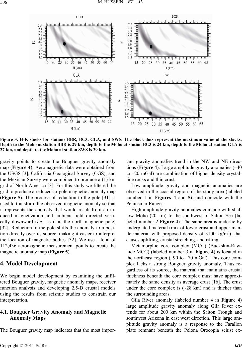

M. HUSSEIN ET AL.
506
Figure 3. H-K stacks for stations BBR, BC3, GLA, and SWS. The black dots represent the maximum value of the stacks.
Depth to the Moho at station BBR is 29 km, depth to the Moho at station BC3 is 24 km, de pth to the Moho at station GLA is
27 km, and depth to the Moho at station SWS is 29 km.
gravity points to create the Bouguer gravity anomaly
map (Figure 4). Aeromagnetic data were obtained from
the USGS [3], California Geological Survey (CGS), and
the Mexican Survey were combined to produce a (1) km
grid of North America [3]. For this study we filtered the
grid to produce a reduced-to-pole magnetic anomaly map
(Figure 5). The process of reduction to the pole [31] is
used to transform the observed magnetic anomaly so that
it represents the anomaly that would result from an in-
duced magnetization and ambient field directed verti-
cally downward (i.e., as if at the north magnetic pole)
[32]. Reduction to the pole shifts the anomaly to a posi-
tion directly over its source, making it easier to interpret
the location of magnetic bodies [32]. We use a total of
112,436 aeromagnetic measurement points to create the
magnetic anomaly map (Figure 5).
4. Model Development
We begin model development by examining the unfil-
tered Bouguer gravity, magnetic anomaly maps, receiver
function analysis and developing 2.5-D crustal models
using the results from seismic studies to constrain our
interpretation.
4.1. Bouguer Gravity Anomaly and Magnetic
Anomaly Maps
The Bouguer gravity map indicates that the most impor-
tant gravity anomalies trend in the NW and NE direc-
tions (Figure 4). Large amplitude gravity ano malies (–40
to –20 mGal) are combination of higher density crystal-
line rocks and thin crust.
Low amplitude gravity and magnetic anomalies are
observed in the coastal region of the study area (labeled
number 1 in Figures 4 and 5), and coincide with the
Peninsular Ranges.
High amplitude gravity anomalies coincide with shal-
low Moho (20 km) to the southwest of Salton Sea (la-
beled number 2 Figure 4). The same area is underlie by
underplated material (mix of lower crust and upper man-
tle material with proposed density of 3100 kg/m3), that
causes uplifting, crustal stretching, and rifting.
Metamorphic core complex (MCC) (Buckskin-Raw-
hide MCC) (labeled number 3 in Figure 4) is located in
the northeast region (–90 to –70 mGal). This core com-
plex lacks a strong Bouguer gravity anomaly. Thus re-
gardless of its source, the material that maintains crustal
thickness beneath the core complex must have approxi-
mately the same density as average crust [16]. The crust
under the core complex is (~28 km) and is thicker than
the surrounding areas.
Gila River anomaly (labeled number 4 in Figure 4)
large amplitude gravity anomaly along Gila River ex-
tends for about 200 km within the Salton Trough and
southwest Arizona in east west direction. This large am-
plitude gravity anomaly is a response to the Farallon
late remnant beneath the Pelona Orocopia schist ex- p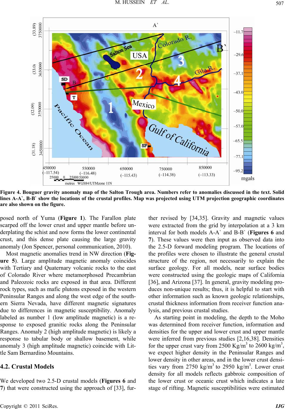

507 M. HUSSEIN ET AL.
Figure 4. Bouguer gravity anomaly map of the Salton Trough area. Numbers refer to anomalies discussed in the text. Solid
lines A-A`, B-B` show the locations of the crustal profiles. Map was projected using UTM projection geographic c oordinates
are also shown on the figure.
posed north of Yuma (Figure 1). The Farallon plate
scarped off the lower crust and upper mantle before un-
derplating the schist an d now forms the lower con tin ental
crust, and this dense plate causing the large gravity
anomaly (Jon Spe ncer , personal commun icat i on, 2 01 0 ).
Most magnetic anomalies trend in NW direction (Fig-
ure 5). Large amplitude magnetic anomaly coincides
with Tertiary and Quaternary volcanic rocks to the east
of Colorado River where metamorphosed Precambrian
and Paleozoic rocks are exposed in that area. Different
rock types, such as mafic plutons exposed in the western
Peninsular Ranges and along the west edge of the south-
ern Sierra Nevada, have different magnetic signatures
due to differences in magnetic susceptibility. Anomaly
labeled as number 1 (low amplitude magnetic) is a re-
sponse to exposed granitic rocks along the Peninsular
Ranges. Anomaly 2 (high amplitude magnetic) is likely a
response to tabular body or shallow basement, while
anomaly 3 (high amplitude magnetic) coincide with Lit-
tle Sam Bernardino Mountains.
4.2. Crustal Models
We developed two 2.5-D crustal models (Figures 6 and
7) that were constructed using the approach of [33], fur-
ther revised by [34,35]. Gravity and magnetic values
were extracted from the grid by interpolation at a 3 km
interval for both models A-A` and B-B` (Figures 6 and
7). These values were then input as observed data into
the 2.5-D forward modeling program. The locations of
the profiles were chosen to illustrate the general crustal
structure of the region, not necessarily to explain the
surface geology. For all models, near surface bodies
were constructed using the geologic maps of California
[36], and Arizona [37]. In general, gravity modeling pro-
duces non-unique results; thus, it is helpful to start with
other information such as known geologic relationships,
crustal thickness information from receiver function ana-
lysis, and previous crustal studies.
As starting point in modeling, the depth to the Moho
was determined from receiver function, information and
densities for the upper and lower crust and upper mantle
were inferred from previous studies [2,16,38]. Densities
for the upper crust vary from 2500 Kg/m3 to 2600 kg/m3,
we expect higher density in the Peninsular Ranges and
lower density in other areas, an d in the lower crust densi-
ties vary from 2750 kg/m3 to 2950 kg/m3. Lower crust
density for all models reflects gabbroic composition of
the lower crust or oceanic crust which indicates a late
tage of rifting. Magnetic susceptibilities were estimated s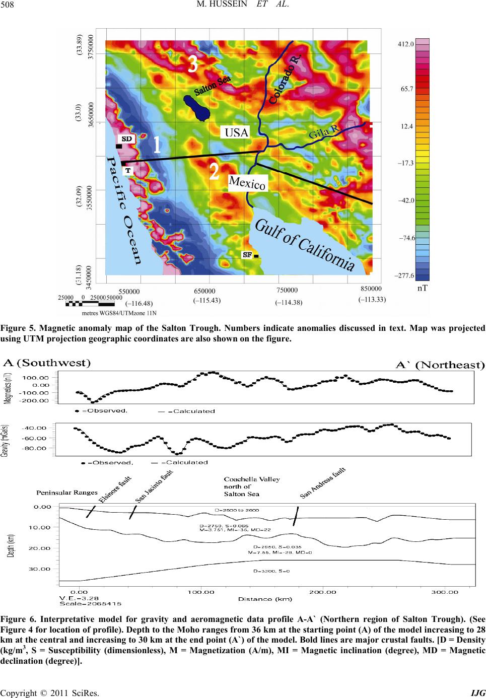

M. HUSSEIN ET AL.
508
Figure 5. Magnetic anomaly map of the Salton Trough. Numbers indicate anomalies discussed in text. Map was projected
using UTM projection geographic coordinates are also shown on the figure.
Figure 6. Interpretative model for gravity and aeromagnetic data profile A-A` (Northern region of Salton Trough). (See
Figure 4 for location of profile). Depth to the Moho ranges from 36 km at the starting point (A) of the model increasing to 28
km at the central and increasing to 30 km at the end point (A`) of the model. Bold lines are major crustal faults. [D = Density
(kg/m3, S = Susceptibility (dimensionless), M = Magnetization (A/m), MI = Magnetic inclination (degree), MD = Magnetic
declination (degree)].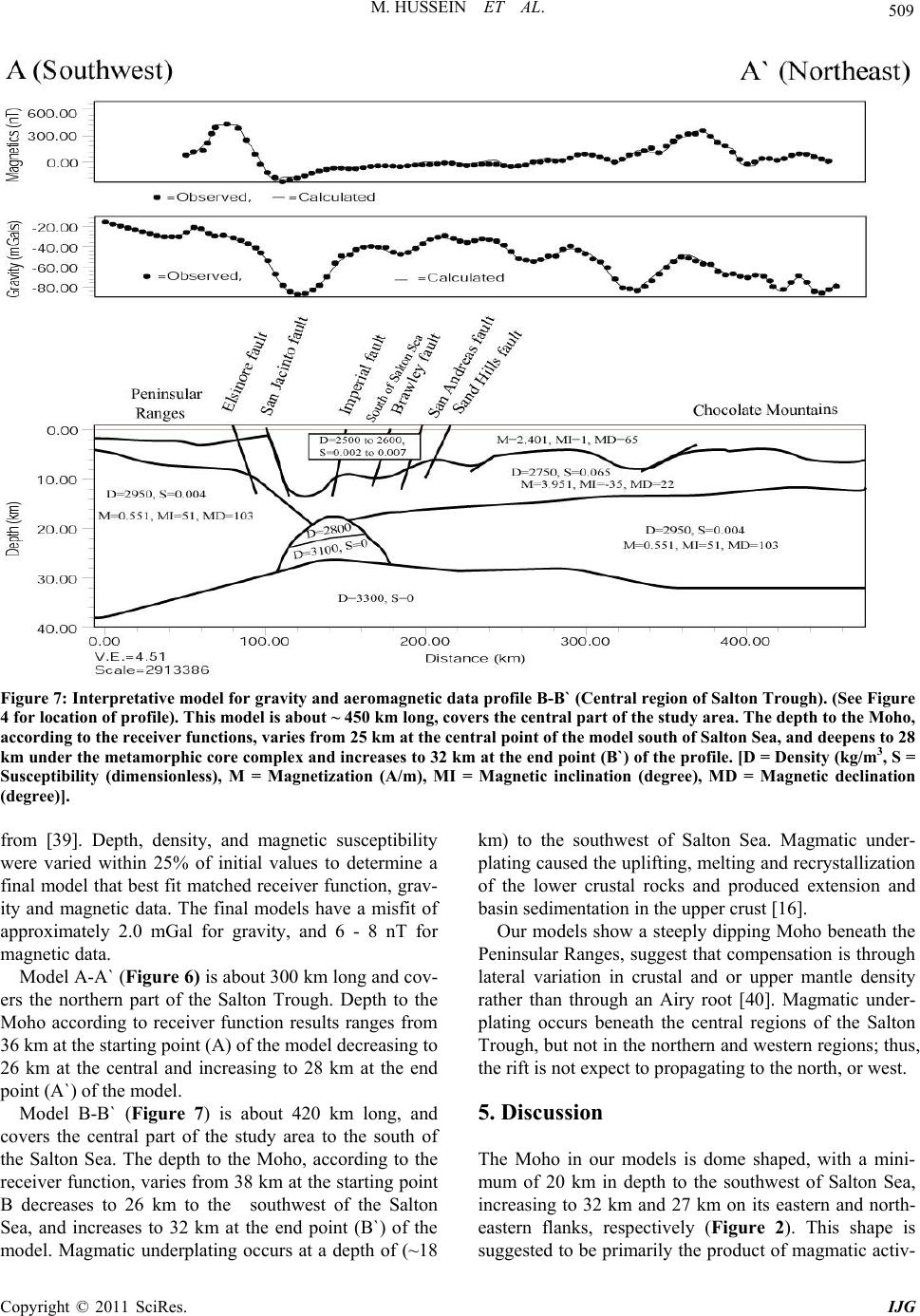

509 M. HUSSEIN ET AL.
Figure 7: Interpretative model for gravity and aeromagnetic data profile B-B` (Central region of Salton Trough). (See Figure
4 for location of profile). This model is about ~ 450 km long, covers the central part of the study area. The depth to the Moho,
according to the receiver functions, varies from 25 km at the central point of the model south of Salton Sea, and deepens to 28
km under the metamorphic core complex and increases to 32 km at the end point (B`) of the profile. [D = Density (kg/m3, S =
Susceptibility (dimensionless), M = Magnetization (A/m), MI = Magnetic inclination (degree), MD = Magnetic declination
(degree)].
from [39]. Depth, density, and magnetic susceptibility
were varied within 25% of initial values to determine a
final model that best fit matched receiver function, grav-
ity and magnetic data. The final models have a misfit of
approximately 2.0 mGal for gravity, and 6 - 8 nT for
magnetic data.
Model A-A` (Figure 6) is about 300 km long and cov-
ers the northern part of the Salton Trough. Depth to the
Moho according to receiver function results ranges from
36 km at the starting point (A) of the model decreasing to
26 km at the central and increasing to 28 km at the end
point (A`) of the model.
Model B-B` (Figure 7) is about 420 km long, and
covers the central part of the study area to the south of
the Salton Sea. The depth to the Moho, according to the
receiver function, varies from 38 km at the starting point
B decreases to 26 km to the southwest of the Salton
Sea, and increases to 32 km at the end point (B`) of the
model. Magmatic underplating occurs at a depth of (~18
km) to the southwest of Salton Sea. Magmatic under-
plating caused the uplifting, melting and recrystallizatio n
of the lower crustal rocks and produced extension and
basin sedimentation in the upper crust [16].
Our models show a steeply dipping Moho beneath the
Peninsular Ranges, suggest that compensation is through
lateral variation in crustal and or upper mantle density
rather than through an Airy root [40]. Magmatic under-
plating occurs beneath the central regions of the Salton
Trough, but not in the northern and western regions; thus,
the rift is not expect to propag ating to the north, or west.
5. Discussion
The Moho in our models is dome shaped, with a mini-
mum of 20 km in depth to the southwest of Salton Sea,
increasing to 32 km and 27 km on its eastern and north-
eastern flanks, respectively (Figure 2). This shape is
suggested to be primarily the product of magmatic activ-

M. HUSSEIN ET AL.
510
ity in the lower crust and upper mantle. Accord ing to our
models the lower crust density ranges from 2750 kg/m3
to 2950 kg/m3. These values represent gabbros, not a
mixture of oceanic and continental crust, while upper
crust densities range from 2500 kg/m3 to 2600 kg/m3.
The large density variation between the upper and lower
crust suggests that the Salton Trough has formed almost
entirely from magmatism in the lower crust and sedi-
mentation in the upper crust as suggested by [2], and
[16].
A large NNW trending gravity and magnetic low (la-
beled number 1; Figures 4 and 5) within the Peninsular
Ranges appears to be related to density contrast in the
lower crust, and upper mantle, indicating the compensa-
tion is through lateral variation in crustal and/or mantle
density rather than through an Airy root [40].
We modeled a magmatic body (mixture of lower crust
and upper mantle material with an assigned density of
3100 kg/m3) model (B-B`) that underlies to the south-
west of the Salton Sea at a depth of about 18 km, and
extends in SW-NE direction for 90 km and extend verti-
cally for about 6 km. We expect this magmatic body
plays a significant role in the process of heating the crust,
stretching and rifting. No evidence for such body to the
north, reference [41] modeled a similar magmatic body
under lower Gila River at depth of 27 km.
6. Conclusions
Incorporation of receiver functions, gravity, and aero-
magnetic data enable us to stud y a broad area of the Sal-
ton Trough to determine its deep structure and answer
important questions regarding the evolution of the Salton
Trough crust. Receiver function analysis suggests the
Moho is 20 km deep to the southwest of the Salton Sea
and deepens to 32 km in the region east of the Salton
Trough. Our models and d ata suggest that the lower crust
of the Salton Trough is oceanic (gabbroic) in composi-
tion, not a mixture of oceanic and continental crust. The
low gravity and low magnetic anomalies observed along
the costal margin of the Salton Trough are an indication
for the absence of Airy root beneath Peninsular Ranges.
Magmatic body exists to the southwest of Salton Sea at
depth of about 18 km, and extends for about 90 km in
SW-NE direction, such body plays a significant role in
heating, stretching and rifting of the crust.
7. Acknowledgements
We would like to thank Dr. Diane Doser, Dr. Terry Pav-
lis, Dr. William Cornell and Dr. Vladik Kreinovich, Dr.
Jon Spencer for helpful discussions. We would like also
to thank Dr. Raed Al-Douri, Carlos Montana for the
technical support. The work was partially supported by
NSF grant number HRD-0734825.
8. References
[1] S. Larsen and R. Reilinger, “Age Constraints for the Pre-
Sent Fault Configuration in the Imperial Valley, Califor-
nia: Evidence for Northwestward Propagation of the Gulf
of California Rift System,” Journal of Geophysical Re-
search, Vol. 96, No. 5624, 1991, pp. 10339-10446.
doi:10.1029/91JB00618
[2] G. Fuis, W. Mooney, J. Healey, G. McMechan and W.
Lutter, “A Seismic Refraction Survey of the Imperial
Valley Region, California,” Journal of Geophysical Re-
search, Vol. 89, No. 2, 1984, pp. 1165-1189.
doi:10.1029/JB089iB02p01165
[3] V. Bankey, A. Cuevas, D. Daniels, C. Finn, I. Hernandez,
P. Hill, R. Kucks,W. Miles, M. Pilkington, C. Roberts, W.
Roest, V. Rystrom, S. Shearer, S. nyder, R. Sweeney, J.
Velez, J. Phillips and D. Ravat, “Digital Data Grids for
the Magnetic Anomaly187 Map of North America,” US
Geological Survey Open-File Report, Denver, 2002.
[4] R. Larson, H. Menard and S. Smith, “Gulf of California:
A Result of Ocean Floor Spreading and Transform Fault-
ing,” Science, Vol. 161, No. 3843, 1968, pp. 781-784.
doi:10.1126/science.161.3843.781
[5] D. Moore and E. Buffington, “Transform Faulting and
Growth of Gulf of California Since the Late Pliocene,”
Science, Vol. 161, No. 3847, 1968, pp. 1238-1241.
doi:10.1126/science.161.3847.1238
[6] W. Elders, R. Rex, T. Mediva, P. Robimson and S.
Biehler, “Crustal Spreading in Southern California,” Sci-
ence, Vol. 178, No. 4056, 1972, pp. 15-24.
doi:10.1126/science.178.4056.15
[7] J. Crowell, “Sedimentation and Tectonics along the San
Andreas Transform Belt,” In: A. G. Sylvester and J. C.
Crowell, Eds., Field Trips for the 28th International
Geological Congress Sedimentation and Tectonics of
North America Belt, American Geophysical Union,
Washington DC, 1989, pp. 32-35.
[8] P. Lonsdale, “Geological and Tectonic History of the
Gulf of California,” In D. Wintere, M. Husson and R.
Decker, Eds., The Eastern Pacifi c Ocean and Hawaii, Geo-
logical Society of America, New York, 1989, pp. 499-521.
[9] J. Stock, and K. Hodges, “Transfer of Baja California to
the Pacific Plate,” Tectonics, Vol. 8, No. 1, 1989, pp. 99-
115. doi:10.1029/TC008i001p00099
[10] G. Axen, M. Grove, D. Stockli, O. Lovera, D. Rothstein,
J. Fletcher, K. Farley and P. Abbott, “Thermal Evolution
of Monte Blanco Dome: Low Angle Normal Faulting
during Gulf of California Rifting and Eocene Denudation
of the Eastern Peninsular Ranges,” Tectonics, Vol. 19, No.
2, 2000. pp. 197-212. doi:10.1029/1999TC001123
[11] D. Karig and W. Jensky, “The Protogulf of California,”
Earth and Planetary Scie nce Letters, Vol. 17, No. 1, 1972,
pp . 1 6 9 -174. doi:10.1016/0012-821X(72)90272-5
[12] D. Moore, “Plate Edge Deformation and Crustal Growth,

511 M. HUSSEIN ET AL.
Gulf of California Structural Province,” Geological Soci-
ety of America Bulletin, Vol. 84, No. 6, 1973, pp.
883-1906.
doi:10.1130/0016-7606(1973)84<1883:PDACGG>2.0.C
O;2
[13] J. Curry and D. Moore, “Geological History of the Mouth
of the Gulf of California,” In: J. K. Crouch and S. B.
Bachmna, Eds., Tectonics and Sedimentary along the
California Margin, Pacific Section, Society of Economic
Paleontologists and Mineralogists, Bakersfield, 1984, pp.
17-36.
[14] R. Gastile, “Proceeding of Conference of Geologic Prob-
lems of the San Andreas Fault System,” Stanford Univer-
sity Publication Geological Sciences, Vol. 11, 1968, pp.
283-286.
[15] R. Dokka and R. Merriam, “Late Cenozoic Extension of
Northeastern Baja California,” Geological Society of
America Bulletin, Vol. 93, No. 5, 1982, pp. 371-378.
doi:10.1130/0016-7606(1982)93<371:LCEONB>2.0.CO;
2
[16] T. Parsons, J. McCarthy and G. Thompson, “Very Differ-
ent Crustal Response to Extreme Extension in the South-
ern Basin and Range and Colorado Plateau Transition,”
In: M. C. Erskine, J. E. Faulds, J. M. Bartley and P. D.
Rowley, Eds., American Association of Petroleum Geolo-
gists Pacific Section Guidebook, Vol. 78, 2001, pp. 291-
304.
[17] A. Gonzalez-Fernandez, J. Danobeitia, L. Delgado-Ar-
gote, F. Michaud, D. Ccrdoba and R. Bartolome, “Mode
of Extension and Rifting History of Upper Tiburón and
Upper Delfín Basins, Northern Gulf of California,”
Journal of Geophysical Research, Vol. 110, 2005, B01313.
[18] D. Lizarralde, G. Axen, H. Brown, J. Fletcher, A. Gon-
zalez-Fernandez, A. Harding, W. Holbrook, G. Kent, P.
Paramo, F. Sutherland and P. Umhoefer, “Variation in
Styles of Rifting in the Gulf of California,” Nature, Vol.
448, 2007, pp. 466-469. doi:10.1038/nature06035
[19] R. Bialas and W. Buck, “How Sediment Promotes Nar-
row Rifting: Application to the Gulf of California,” Tec-
tonics, Vol. 28, 2009, TC4014.
doi:10.1029/2008TC002394
[20] R. Dorsey, “Sedimentation and Crustal Recycling along
an Active Oblique-Rift Margin: Salton Trough and North-
ern Gulf of California,” Geological Society of America,
Vol. 38, 2010, pp. 443-446.
[21] C. Ammon, G. Randall and G. Zandt, “On the Nonuni-
queness of Receiver Function Inversions,” Journal of
Geophysical Research, Vol. 95, 1990, pp.15303-15318.
[22] L. Zhu and H. Kanamori, “Moho Depth Variation in
Southern California from Teleseimic Receiver Function,”
Journal of Geophysical Research, Vol. 105, No. B2, 2000,
pp. 2969-2980. doi:10.1029/1999JB900322
[23] J. Ligorria and G. Ammon, “Iterative Deconvolution and
Receiver Functions Estimation,” Bulletin of Seismologi-
cal Society of America, Vol. 89, 1999, pp. 1395-1400.
[24] L. Zhu, “Estimation of Crustal Thickness and Vp/Vs
Ratio beneath the Tibetan Plateau from Teleseismic
Converted Waves (Abstract),” Eos Transactions Ameri-
can Geophysical Union, Vol. 74, No. 16, 1993, p. 202.
[25] G. Zandt, S. Myers and T. Wallace, “Crust and Mantle
Structure across the Basin and Range Colorado Plateau
Boundary at 37˚N Latitude and Implication for Cenozoic
Extensional Mechanism,” Journal of Geophysical Re-
search, Vol. 100, No. B6, 1995, pp. 10529-10548.
doi:10.1029/94JB03063
[26] G. Zandt and C. Ammon, “Continental Crust Composi-
tion Constrained by Measurements of Crustal Poisson
Ratio,” Nature, Vol. 374, No. 6518, 1995, pp. 152-154.
doi:10.1038/374152a0
[27] D. Eaton, S. Dineva and R. Mereu, “Crustal Thickness
and Vp/Vs Variations in the Grenville Orogen (Ontario,
Canada) from Analysis of Teleismic Receiver Function,”
Tectonophysics, Vol. 420, No. 1-2, 2006, pp. 223-238.
doi:10.1016/j.tecto.2006.01.023
[28] T. Nakajima, T. Matsuzawa, A. Hasegawa and D. Zaho,
“Three Dimensional Structure of Vp, Vs, and Vp/Vs be-
neath Northeastern Japan: Implications for Arc Magma-
tism and Fluids,” Journal of Geophysical Research, Vol.
106, No. B10, 2001, pp. 21843-21857.
doi:10.1029/2000JB000008
[29] M. Webring, “MINC, a Gridding Program Based on
Minimum Curvature,” US Geological Survey Open-File
Report 81-1224, 1982, p. 43.
[30] D. Plouff, “Preliminary Documentation for a Fortran
Program to Compute Gravity Terrain Corrections Based
on Topography Digitized on a Geographic Grid,” US
Geological Survey Open File Report 77-535, 1977, p. 45.
[31] B. Baranov and H. Naudy, “Numerical Calculation of the
Formula of Reduction to the Magnetic Pole,” Geophysics,
Vol. 29, No. 1, 1964. pp. 67-79.
doi:10.1190/1.1439334
[32] R. Blakely, “Potential Theory in Gravity and Magnetic
Applications,” Cambridge University Press, New York,
1995. doi:10.1017/CBO9780511549816
[33] M. Talwani, J. Worzel and M. Landisman, “Rapid Grav-
ity Computations for Two-Dimensional Bodies with Ap-
plication to the Mendocino Submarine Fracture Zone,”
Journal of Geophysical Research, Vol. 64, No. 1, 1959,
pp. 49-59. doi:10.1029/JZ064i001p00049
[34] L. Pedersen, “Interpretation of Potential Field Data, a
Generalized Inverse Approach,” Geophysical Prospecting,
Vol. 25, No. 2, 1977. pp. 199-230.
doi:10.1111/j.1365-2478.1977.tb01164.x
[35] J. Cady, “Calculation of Gravity and Magnetic Anomalies
of Finite-Length Right Polygonal Prisms,” Geophysics,
Vol. 45, No. 10, 1980, pp. 1507-1512.
doi:10.1190/1.1441045
[36] C. Jennings, “Geologic Map of California. Scale 1: 750,000,
California,” Department of Mines and Geology, 1997.
[37] S. Reynolds, “Geological Map of Arizona. Scale 1:
1,000,000,” Arizona Geological Survey, 1988.
[38] T. Parsons and T. McCarthy, “Crustal and Upper Mantle
Velocity Structure of the Salton Trough Southeast Cali-

M. HUSSEIN ET AL.
512
fornia,” Tectonics, Vol. 15, No. 2, 1996, pp. 456-471.
doi:10.1029/95TC02616
[39] V. Langenheim, R. Jachen, J. Matti, E. Hauksson, D.
Morton and A. Christensen, “Geophysical Evidence for
Wedging in the San Gergonio Pass Structural Knot,
Southern San Andreas Fault Zone, Southern California,”
GSA Bulletin, Vol. 117, No. 110, 2005. pp. 1554-1572.
doi:10.1130/B25760.1
[40] J. Lewis, S. Day, H. Magistrale, J. Ealins and F. Vernon,
“Regional Crustal Variations off the Peninsular Ranges,
Southern California,” Geology, Vol. 28, No. 4, 2000, pp.
303-306.
doi:10.1130/0091-7613(2000)28<303:RCTVOT>2.0.CO;
2
[41] M. Hussein, “Integrated and Comparative Geophysical
Studies of Crustal Structure of Pull-Apart Basins: The
Salton Trough and Death Valley, California Regions,”
Ph.D. Dissertation, University of Texas at El Paso, El
Paso, 2007.
[42] R. Dorsey, “Stratigraphic Record of Pleistocene Initiation
and Slip on the Coyote Creek Fault, Lower Southern
California,” In: A. Bath, Ed., Contributions to Crustal
evolution of the southwest United States, Geological So-
ciety of America, 2002, pp. 251-269.
Websites
NSF, “Earthscope,” 2006. http//www. earthscope.org/
NS F, “Earthscop e Automated Receivers Survey (EARS),”
2006. http://www.ears.iris.washington.edu
UTEP, “Pan-American Center for Earth and Environ-
mental Studies,” 2006. http://research.utep.edu/ paces