International Journal of Geosciences, 2011, 2, 457-467
doi:10.4236/ijg.2011.24048 Published Online November 2011 (http://www.SciRP.org/journal/ijg)
457
Comparative Study of Analytical Solutions for
Time-Dependent Solute Transport along Unsteady
Groundwater Flow in Semi-infinite Aquifer
Mritunjay Kumar Singh*, Nav Kumar Mahato, Priyanka Kumari
Department of Ap pl i e d Mat hematics, Indian School of Mines, Dhanbad, India
Received June 29, 2011; revised August 6, 2011; accepted September 12, 2011
Abstract
A comparative study is made among Laplace Transform Technique (LTT) and Fourier Transform Technique
(FTT) to obtain one-dimensional analytical solution for conservative solute transport along unsteady ground-
water flow in semi-infinite aquifer. The time-dependent source of contaminant concentration is considered at
the origin and at the other end of the aquifer is supposed to be zero. Initially, aquifer is not solute free which
means that the solute concentration exits in groundwater system and it is assumed as a uniform concentration.
The aquifer is considered homogeneous and semi-infinite. The time-dependent velocity expressions are con-
sidered. The result may be used as preliminary predictive tools in groundwater management and benchmark
the numerical code and solutions.
Keywords: Solute Transport, Unsteady, Aquifer, Analytical Solutions
1. Introduction
As we know, groundwater constituents are an important
component of many natural water resource systems
which supply water for domestic, industrial and agricul-
tural purposes. It is generally a good source of drinking
water. It is believed that groundwater is more risk free in
compare to the surface water. But these days pollution of
groundwater is growing continuously in the various de-
veloping countries particularly India due to the indis-
criminate discharge of waste water from the various in-
dustries, especially coal based industries, which do not
have sufficient treatment facilities. These industries dis-
charge their waste water into the neighboring ponds,
streams; rivers etc. The chemical constituents of the waste
material often infiltrate from these ponds and mixed with
the groundwater system causes groundwater contamina-
tion [1-4]. Groundwater modeling is specially used in the
hydrological sciences for the assessment of the resource
potential and prediction of future impact under different
conditions. Many experimental and theoretical studies
were undertaken to improve the understanding, manage-
ment, and prediction of the movement of contaminant
behavior in groundwater system. These investigations are
primarily motivated by concerns about possible contami-
nation of the subsurface environment. Hydrologist, Civil
engineers, Scientists etc. are doing their best to solve this
type of serious problem by various means. The subsur-
face solute transport is generally described with the ad-
vection-diffusion (AD) equation. In the deterministic
approach, explicit closed-form solutions for transport
problem can often be derived if the model parameters are
constant with respect to time and position [5]. Mathe-
matical modelling is one of the powerful tools to project
the existing problems and its appropriate solutions. Al-
though many transport problems must be solved numeri-
cally, analytical solutions are still pursued by many sci-
entists because they can provide better physical insight
into problems. Groundwater transport and its mathemati-
cal models were presented significantly [6-11]. Analyti-
cal approach of solute transport problems in ground-
water reservoirs is explored [12-14]. In the present work,
our objective is to find the analytical solutions using
Fourier Transform Technique (FTT) and to compare the
result with the solution obtained by Laplace Transform
Technique (LTT). To predict the nature of the contami-
nant concentration along unsteady groundwater flow in
semi-infinite aquifer, a comparative study is made by the
proposed methods. Time-dependent velocity expres-
sions are considered to illustrate the obtained result.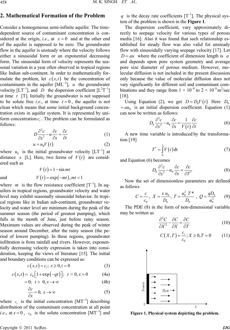

M. K. SINGH ET AL.
458
2. Mathematical Formation of the Problem
Consider a homogeneous semi-infinite aquifer. The time-
dependent source of contaminant concentration is con-
sidered at the origin, i.e., at 0x and at the other end
of the aquifer is supposed to be zero. The groundwater
flow in the aquifer is unsteady where the velocity follows
either a sinusoidal form or an exponential decreasing
form. The sinusoidal form of velocity represents the sea-
sonal variation in a year often observed in tropical regions
like Indian sub-continent. In order to mathematically for-
mulate the problem, let


,cxt be the concentration of
contaminants in the aquifer [ML–3], u the groundwater
velocity [LT–1], and D the dispersion coefficient [L2T–1]
at time t [T]. Initially the groundwater is not supposed
to be solute free i.e., at time 0t, the aquifer is not
clean which means that some initial background concen-
tration exists in aquifer system. It is represented by uni-
form concentrationi c. The problem can be formulated as
follows:
2
2
ccc
Du
x
t
x


  (1)

0
uuVt (2)
where 0
u is the initial groundwater velocity [LT–1] at
distance
x
[L]. Here, two forms of

Vt are consid-
ered such as

1sinVt mt
and



exp, 1Vtmt mt 
where m is the flow resistance coefficient [T–1]. In aq-
uifers in tropical regions, groundwater velocity and water
level may exhibit seasonally sinusoidal behavior. In tropi-
cal regions like in Indian sub-continent, groundwater ve-
locity and water level are minimum during the peak of the
summer season (the period of greatest pumping), which
falls in the month of June, just before rainy season.
Maximum values are observed during the peak of winter
season around December, after the rainy season (the pe-
riod of lowest pumping). In these regions, groundwater
infiltration is from rainfall and rivers. However, exponen-
tially decreasing velocity expression is taken into consi-
deration, keeping the views of literature [15]. The initial
and boundary conditions can be expressed as:

,; 0,0
i
cxtc xt (3)
 
0
, 1exp; > 0,0 cxt cqttx
 (4a)
0; 0, tx (4b)
0;
cx
x

 (5)
where i
c is the initial concentration [MT–3] describing
distribution of the contaminant concentration at all point
i.e., at0x, 0
c is the solute concentration [MT–3] and
q is the decay rate coefficients [T–1]. The physical sys-
tem of the problem is shown in the Figure 1.
The dispersion coefficient, vary approximately di-
rectly to seepage velocity for various types of porous
media [16]. Also it was found that such relationship es-
tablished for steady flow was also valid for unsteady
flow with sinusoidally varying seepage velocity [17]. Let
Dau

where the coefficient of dimension length is a
and depends upon pore system geometry and average
pore size diameter of porous medium. However, mo-
lecular diffusion is not included in the present discussion
only because the value of molecular diffusion does not
vary significantly for different soil and contaminant com-
binations and they range from 1 × 10–9 to 2 × 10–9 m2/sec
[18].
Using Equation (2), we get

0
DDVt Here 0 D
0
au

is an initial dispersion coefficient. Equation (1)
can now be written as follows:

2
00
2
1cc c
Du
x
Vt tx




 (6)
A new time variable is introduced by the transforma-
tion [19]

*
0
dt
t
TVt (7)
and Equation (6) becomes
2
00
2*
ccc
Du
x
x
T





 (8)
Now the set of dimensionless parameters are defined
as follows
2
00 0
2
00 00
*
,, ,
x
uuT qD c
CX TQ
cD Du
 
(9)
The PDE (8) in the form of non-dimensional variable
may be written as
2
2
CCC
X
T
X




 (10)

0
,;0,0
i
c
CXTX T
c

(11)
Figure 1. Physical system depicting the problem.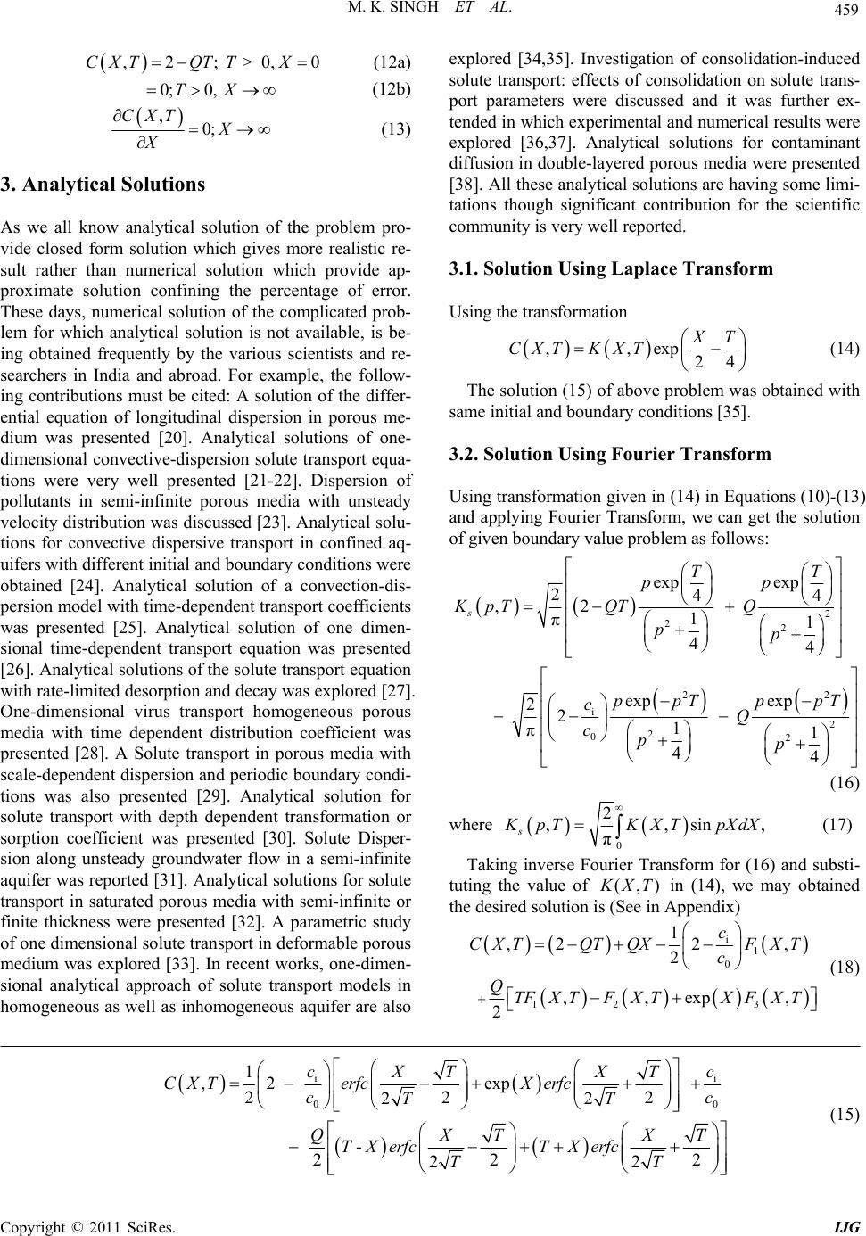

M. K. SINGH ET AL.
459

,2; > 0, 0 CXTQTT X (12a)
0;0, TX 
(12b)

,0; CXT X
X

 (13)
3. Analytical Solutions
As we all know analytical solution of the problem pro-
vide closed form solution which gives more realistic re-
sult rather than numerical solution which provide ap-
proximate solution confining the percentage of error.
These days, numerical solution of the complicated prob-
lem for which analytical solution is not available, is be-
ing obtained frequently by the various scientists and re-
searchers in India and abroad. For example, the follow-
ing contributions must be cited: A solution of the differ-
ential equation of longitudinal dispersion in porous me-
dium was presented [20]. Analytical solutions of one-
dimensional convective-dispersion solute transport equa-
tions were very well presented [21-22]. Dispersion of
pollutants in semi-infinite porous media with unsteady
velocity distribution was discussed [23]. Analytical solu-
tions for convective dispersive transport in confined aq-
uifers with different initial and boundary conditions were
obtained [24]. Analytical solution of a convection-dis-
persion model with time-dependent transport coefficients
was presented [25]. Analytical solution of one dimen-
sional time-dependent transport equation was presented
[26]. Analytical solutions of the solute transport equation
with rate-limited desorption and decay was explored [27].
One-dimensional virus transport homogeneous porous
media with time dependent distribution coefficient was
presented [28]. A Solute transport in porous media with
scale-dependent dispersion and periodic boundary condi-
tions was also presented [29]. Analytical solution for
solute transport with depth dependent transformation or
sorption coefficient was presented [30]. Solute Disper-
sion along unsteady groundwater flow in a semi-infinite
aquifer was reported [31]. Analytical solutions for solute
transport in saturated porous media with semi-infinite or
finite thickness were presented [32]. A parametric study
of one dimensional solute transport in deformable porous
medium was explored [33]. In recent works, one-dimen-
sional analytical approach of solute transport models in
homogeneous as well as inhomogeneous aquifer are also
explored [34,35]. Investigation of consolidation-induced
solute transport: effects of consolidation on solute trans-
port parameters were discussed and it was further ex-
tended in which experimental and numerical results were
explored [36,37]. Analytical solutions for contaminant
diffusion in double-layered porous media were presented
[38]. All these analytical solutions are having some limi-
tations though significant contribution for the scientific
community is very well reported.
3.1. Solution Using Laplace Transform
Using the transformation

,,exp
24
X
T
CXTKXT 


(14)
The solution (15) of above problem was obtained with
same initial and boundary conditions [35].
3.2. Solution Using Fourier Transform
Using transformation given in (14) in Equations (10)-(13)
and applying Fourier Transform, we can get the solution
of given boundary value problem as follows:
 
 
2
22
22
i
2
2
02
exp exp
244
,2
1 π1
44
exp exp
2
2
1
π1
44
s
TT
pp
KpT QTQ
pp
ppT ppT
cQ
cpp


 


 
 


 



















 



 
 




 


(16)
where
 
0
2
,,sin,
π


s
K
pTKXTpXdX (17)
Taking inverse Fourier Transform for (16) and substi-
tuting the value of (,)
K
XT in (14), we may obtained
the desired solution is (See in Appendix)

 
i
1
0
12 3
1
,22 ,
2
,,exp,
2
c
CXTQT QXFXT
c
QTFXTFX TXFXT










(18)
 
 
i i
0 0
1
,2 exp
22 2
22
-
22 2
22
ccXT XT
CXT erfcXerfc
cc
TT
QXTXT
TXerfcT Xerfc
TT

 

 
  

 


 


 

  
 

 

(15)

M. K. SINGH ET AL.
460
where


1,22
exp22
TX
FXT erfcT
TX
Xerfc T










(18a)

2
2
,22
2
exp2
π2














TX
FXT XerfcT
TTX
T
(18b)

3
2
,22
2
exp2
π2














TX
FXT XerfcT
TTX
T
(18c)
4. Illustration and Discussion
We consider the sinusoidally varying and exponentially
decreasing forms of velocities which are valid fortran-
sient groundwater flow too [15, 23]. Now from Equation
(2) the velocity expressions are as follows:
 
01sinutumt (19a)

0exp, 1utumt mt (19b)
where m(/day) is the flow resistance coefficient. For both
the expressions, the non-dimensional time variable T
may be written as

2
0
0
1cos
u
Tmt mt
mD


(20a)

2
0
0
1exp
u
Tmt
mD




 (20b)
where mt = 3k + 2, k is a whole number are chosen. For
m = 0.0165 (/day), (19a) yields, t (days) =182k + 121,
approximately. For these values of mt, the velocity u, is
alternatively minimum and maximum. Hence it repre-
sents the groundwater level and velocity minimum dur-
ing the month of June and maximum during December
just after six months (Approximately 182 days) in one
year. The next data of t represents minimum and maxi-
mum records during June and December respectively in
the subsequent years. The sinusoidally varying and ex-
ponentially decreasing form of velocity representations
are made graphically with respect to time at different
values of seepage velocity and dispersion parameters and
shown in the Figures 2(a) and (b). As we increase the
seepage velocity parameter, the peak of sinusoidal form
of velocity increases which reveals in Figure 2(a). This
representation can often be observed in tropical region of
India. An analytical solutions (15) and (18) are computed
for the values ci = 0.1, c0 = 1.0, u0 = 0.033 - 0.045 km/day,
D0 = 0.33 - 0.45 km2/day, q = 0.0009(/day), and
x
= 10
km. The time-dependent concentration values are de-
picted from the table 1(a-d) for sinusoidal form of veloc-
ity expression 19(a) at the seepage velocity u
0 ranging
from 0.033 km/day to 0.042 km/day and dispersions pa-
rameter D0 ranging from 0.33 km2/day to 0.42 km2/day.
The concentration values at different positions are ob-
tained for both the methods LTT and FTT in row (i) and
row (ii) respectively shown in Tables 1and 2. It is ob-
served that concentration values decreases rapidly in row
(i) in comparison to row (ii). However, in Tab les 3 and 4
the concentration values also decreases rapidly in row (i)
and slowly and gradually converges at a common point
15001600 1700 1800 1900 2000 2100 2200 2300 2400 2500
0
0.01
0.02
0.03
0.04
0.05
0.06
0.07
0.08
0.09
Time
(
da
y
s
)
Sinusoidal Velocity(km/day)
3
4
2
1
S.I.No. Seepage Velocity
u
0
(km/day)
1 0.033
2 0.036
3 0.039
4 0.042
1500 1600 17001800 190020002100 2200 230024002500
0.02
0.022
0.024
0.026
0.028
0.03
0.032
Time(days)
Exponential Decreasing Velocity(km/day)
4
3
2
1
S.I.No. Seepage Velocity
u
0
(km/day)
1 0.033
2 0.036
3 0.039
4 0.042
(a) (b)
Figure 2. Time-dependent (a) sinusoidally varying velocity and (b) exponentially decreasing velocity representations subject
to seepage velocity u0 = 0.033 - 0.045 km/day. Curves No. 1 - 5 represent the contaminant concentrations in 5th year, 6th year,
and 7th year December and June, respectively.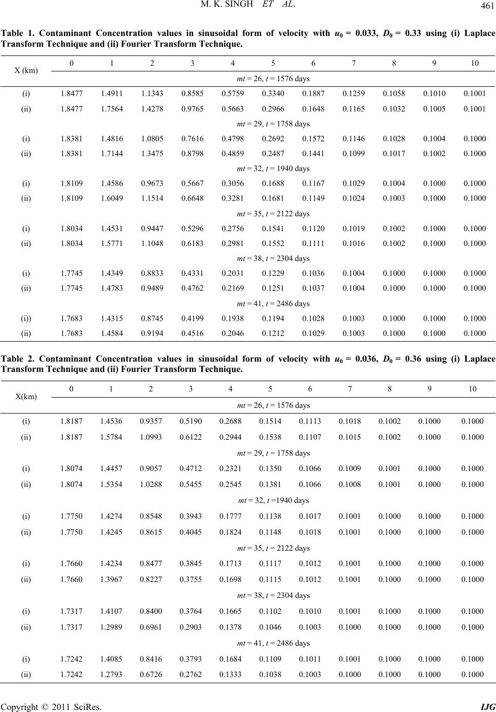

M. K. SINGH ET AL.
461
Table 1. Contaminant Concentration values in sinusoidal form of velocity with u0 = 0.033, D0 = 0.33 using (i) Laplace
Transform Technique and (ii) Fourier Tr ansfor m Tec hnique.
0 1 2 3 4 5 6 7 8 9 10
X (km) mt = 26, t = 1576 days
(i) 1.8477 1.4911 1.1343 0.8585 0.5759 0.3340 0.1887 0.1259 0.1058 0.1010 0.1001
(ii) 1.8477 1.7564 1.4278 0.9765 0.5663 0.2966 0.1648 0.1165 0.1032 0.1005 0.1001
mt = 29, t = 1758 days
(i) 1.8381 1.4816 1.0805 0.7616 0.4798 0.2692 0.1572 0.1146 0.1028 0.1004 0.1000
(ii) 1.8381 1.7144 1.3475 0.8798 0.4859 0.2487 0.1441 0.1099 0.1017 0.1002 0.1000
mt = 32, t = 1940 days
(i) 1.8109 1.4586 0.9673 0.5667 0.3056 0.1688 0.1167 0.1029 0.1004 0.1000 0.1000
(ii) 1.8109 1.6049 1.1514 0.6648 0.3281 0.1681 0.1149 0.1024 0.1003 0.1000 0.1000
mt = 35, t = 2122 days
(i) 1.8034 1.4531 0.9447 0.5296 0.2756 0.1541 0.1120 0.1019 0.1002 0.1000 0.1000
(ii) 1.8034 1.5771 1.1048 0.6183 0.2981 0.1552 0.1111 0.1016 0.1002 0.1000 0.1000
mt = 38, t = 2304 days
(i) 1.7745 1.4349 0.8833 0.4331 0.2031 0.1229 0.1036 0.1004 0.1000 0.1000 0.1000
(ii) 1.7745 1.4783 0.9489 0.4762 0.2169 0.1251 0.1037 0.1004 0.1000 0.1000 0.1000
mt = 41, t = 2486 days
(i)) 1.7683 1.4315 0.8745 0.4199 0.1938 0.1194 0.1028 0.1003 0.1000 0.1000 0.1000
(ii) 1.7683 1.4584 0.9194 0.4516 0.2046 0.1212 0.1029 0.1003 0.1000 0.1000 0.1000
Table 2. Contaminant Concentration values in sinusoidal form of velocity with u0 = 0.036, D0 = 0.36 using (i) Laplace
Transform Technique and (ii) Fourier Tr ansfor m Tec hnique.
0 1 2 3 4 5 6 7 8 9 10
X(km) mt = 26, t = 1576 days
(i) 1.8187 1.4536 0.9357 0.5190 0.2688 0.1514 0.1113 0.1018 0.1002 0.1000 0.1000
(ii) 1.8187 1.5784 1.0993 0.6122 0.2944 0.1538 0.1107 0.1015 0.1002 0.1000 0.1000
mt = 29, t = 1758 days
(i) 1.8074 1.4457 0.9057 0.4712 0.2321 0.1350 0.1066 0.1009 0.1001 0.1000 0.1000
(ii) 1.8074 1.5354 1.0288 0.5455 0.2545 0.1381 0.1066 0.1008 0.1001 0.1000 0.1000
mt = 32, t =1940 days
(i) 1.7750 1.4274 0.8548 0.3943 0.1777 0.1138 0.1017 0.1001 0.1000 0.1000 0.1000
(ii) 1.7750 1.4245 0.8615 0.4045 0.1824 0.1148 0.1018 0.1001 0.1000 0.1000 0.1000
mt = 35, t = 2122 days
(i) 1.7660 1.4234 0.8477 0.3845 0.1713 0.1117 0.1012 0.1001 0.1000 0.1000 0.1000
(ii) 1.7660 1.3967 0.8227 0.3755 0.1698 0.1115 0.1012 0.1001 0.1000 0.1000 0.1000
mt = 38, t = 2304 days
(i) 1.7317 1.4107 0.8400 0.3764 0.1665 0.1102 0.1010 0.1001 0.1000 0.1000 0.1000
(ii) 1.7317 1.2989 0.6961 0.2903 0.1378 0.1046 0.1003 0.1000 0.1000 0.1000 0.1000
mt = 41, t = 2486 days
(i) 1.7242 1.4085 0.8416 0.3793 0.1684 0.1109 0.1011 0.1001 0.1000 0.1000 0.1000
(ii) 1.7242 1.2793 0.6726 0.2762 0.1333 0.1038 0.1003 0.1000 0.1000 0.1000 0.1000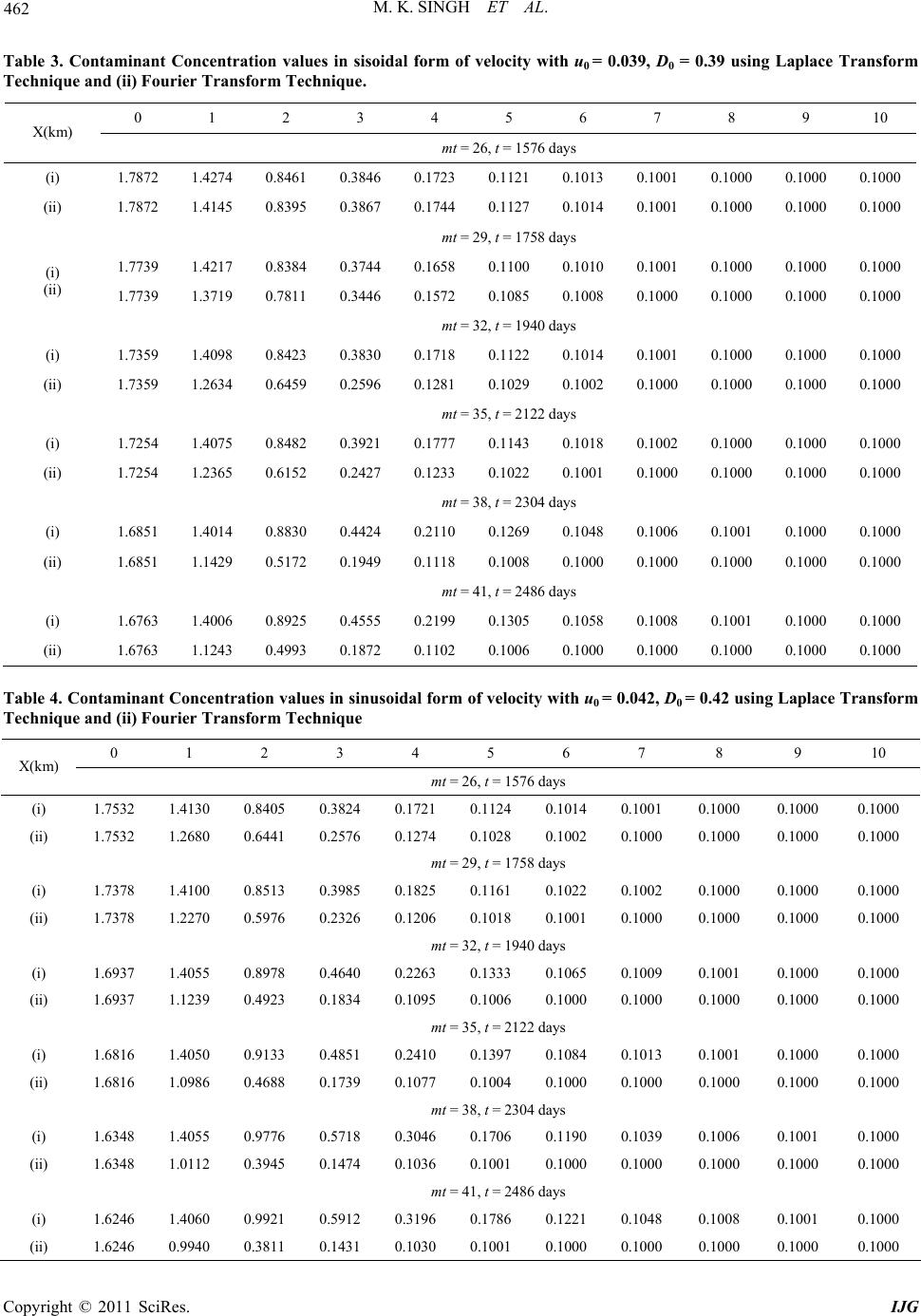

M. K. SINGH ET AL.
462
Table 3. Contaminant Concentration values in sisoidal form of velocity with u0 = 0.039, D0 = 0.39 using Laplace Transform
Technique and (ii) Fourier Transfor m Technique.
0 1 2 3 4 5 6 7 8 9 10
X(km) mt = 26, t = 1576 days
(i) 1.7872 1.4274 0.8461 0.3846 0.1723 0.1121 0.1013 0.1001 0.1000 0.1000 0.1000
(ii) 1.7872 1.4145 0.8395 0.3867 0.1744 0.1127 0.1014 0.1001 0.1000 0.1000 0.1000
mt = 29, t = 1758 days
1.7739 1.4217 0.8384 0.3744 0.1658 0.1100 0.1010 0.1001 0.1000 0.1000 0.1000
(i)
(ii) 1.7739 1.3719 0.7811 0.3446 0.1572 0.1085 0.1008 0.1000 0.1000 0.1000 0.1000
mt = 32, t = 1940 days
(i) 1.7359 1.4098 0.8423 0.3830 0.1718 0.1122 0.1014 0.1001 0.1000 0.1000 0.1000
(ii) 1.7359 1.2634 0.6459 0.2596 0.1281 0.1029 0.1002 0.1000 0.1000 0.1000 0.1000
mt = 35, t = 2122 days
(i) 1.7254 1.4075 0.8482 0.3921 0.1777 0.1143 0.1018 0.1002 0.1000 0.1000 0.1000
(ii) 1.7254 1.2365 0.6152 0.2427 0.1233 0.1022 0.1001 0.1000 0.1000 0.1000 0.1000
mt = 38, t = 2304 days
(i) 1.6851 1.4014 0.8830 0.4424 0.2110 0.1269 0.1048 0.1006 0.1001 0.1000 0.1000
(ii) 1.6851 1.1429 0.5172 0.1949 0.1118 0.1008 0.1000 0.1000 0.1000 0.1000 0.1000
mt = 41, t = 2486 days
(i) 1.6763 1.4006 0.8925 0.4555 0.2199 0.1305 0.1058 0.1008 0.1001 0.1000 0.1000
(ii) 1.6763 1.1243 0.4993 0.1872 0.1102 0.1006 0.1000 0.1000 0.1000 0.1000 0.1000
Table 4. Contaminant Concentration values in sinusoidal form of velocity with u0 = 0.042, D0 = 0.42 using Laplace Transform
Technique and (ii) Fourier Transfor m Technique
0 1 2 3 4 5 6 7 8 9 10
X(km) mt = 26, t = 1576 days
(i) 1.7532 1.4130 0.8405 0.3824 0.1721 0.1124 0.1014 0.1001 0.1000 0.1000 0.1000
(ii) 1.7532 1.2680 0.6441 0.2576 0.1274 0.1028 0.1002 0.1000 0.1000 0.1000 0.1000
mt = 29, t = 1758 days
(i) 1.7378 1.4100 0.8513 0.3985 0.1825 0.1161 0.1022 0.1002 0.1000 0.1000 0.1000
(ii) 1.7378 1.2270 0.5976 0.2326 0.1206 0.1018 0.1001 0.1000 0.1000 0.1000 0.1000
mt = 32, t = 1940 days
(i) 1.6937 1.4055 0.8978 0.4640 0.2263 0.1333 0.1065 0.1009 0.1001 0.1000 0.1000
(ii) 1.6937 1.1239 0.4923 0.1834 0.1095 0.1006 0.1000 0.1000 0.1000 0.1000 0.1000
mt = 35, t = 2122 days
(i) 1.6816 1.4050 0.9133 0.4851 0.2410 0.1397 0.1084 0.1013 0.1001 0.1000 0.1000
(ii) 1.6816 1.0986 0.4688 0.1739 0.1077 0.1004 0.1000 0.1000 0.1000 0.1000 0.1000
mt = 38, t = 2304 days
(i) 1.6348 1.4055 0.9776 0.5718 0.3046 0.1706 0.1190 0.1039 0.1006 0.1001 0.1000
(ii) 1.6348 1.0112 0.3945 0.1474 0.1036 0.1001 0.1000 0.1000 0.1000 0.1000 0.1000
mt = 41, t = 2486 days
(i) 1.6246 1.4060 0.9921 0.5912 0.3196 0.1786 0.1221 0.1048 0.1008 0.1001 0.1000
(ii) 1.6246 0.9940 0.3811 0.1431 0.1030 0.1001 0.1000 0.1000 0.1000 0.1000 0.1000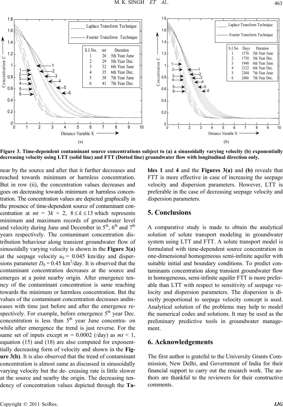

M. K. SINGH ET AL.
463
0 1 23 45 6 78910
0
0. 2
0. 4
0. 6
0. 8
1
1. 2
1. 4
1. 6
1. 8
Distance Variable X
Concentration C
34
56
_______ Laplace Transform Technique
---------- Fourier Transform Technique
3
4
5
2
S.I.No. mt Duration
1 26 5th Year June
2 29 5th Year Dec.
3 32 6th Year June
4 35 6th Year Dec.
5 38 7th Year June
6 41 7th Year Dec.
1
6
1
2
0 1 23 45 6 78 910
0
0. 2
0. 4
0. 6
0. 8
1
1. 2
1. 4
1. 6
1. 8
Distance Variable X
Concentration C
S.I.No Days Duration
1 1576 5th Year June
2 1758 5th Year Dec.
3 1940 6th Year June
4 2122 6th Year Dec.
5 2304 7th Year June
6 2486 7th Year Dec.
1
2
3
5
4
6
2
3456
1
______ Laplace Transform Technique
--------- Fourier Transform Technique
(a) (b)
Figure 3. Time-dependent contaminant source concentrations subject to (a) a sinusoidally varying velocity (b) exponentially
decreasing velocity using LTT (solid line) and FTT (Dotted line) groundwater flow with longitudinal direction only.
near by the source and after that it further decreases and
reached towards minimum or harmless concentration.
But in row (ii), the concentration values decreases and
goes on decreasing towards minimum or harmless concen-
tration. The concentration values are depicted graphically in
the presence of time-dependent source of contaminant con-
centration at mt = 3k + 2, 813k

which represents
minimum and maximum records of groundwater level
and velocity during June and December in 5th, 6th and 7th
years respectively. The contaminant concentration dis-
tribution behaviour along transient groundwater flow of
sinusoidally varying velocity is shown in the Figure 3(a)
at the seepage velocity u
0 = 0.045 km/day and disper-
sions parameter D0 = 0.45 km2/day. It is observed that the
contaminant concentration decreases at the source and
emerges at a point nearby origin. After emergence ten-
ncy of the contaminant concentration is same reaching
towards the minimum or harmless concentration. But the
values of the contaminant concentration decreases andin-
eases with time just before and after the emergence re-
spectively. For example, before emergence 5th year Dec.
concentration is less than 5th year June concentra- on
while after emergence the trend is just reverse. For the
same set of inputs except m = 0.0002 (/day) as mt < 1,
equation (15) and (18) are also computed for exponent-
tially decreasing form of velocity and shown in the Fig-
ure 3(b). It is also observed that the trend of contaminant
concentration is almost same as discussed in sinusoidally
varying velocity but the de- creasing rate is little slower
at the source and nearby the origin. The decreasing ten-
dency of concentration values depicted through the Ta-
bles 1 and 4 and the Figures 3(a) and (b) reveals that
FTT is more effective in case of increasing the seepage
velocity and dispersion parameters. However, LTT is
preferable in the case of decreasing seepage velocity and
dispersion parameters.
5. Conclusions
A comparative study is made to obtain the analytical
solution of solute transport modeling in groundwater
system using LTT and FTT. A solute transport model is
formulated with time-dependent source concentration in
one-dimensional homogeneous semi-infinite aquifer with
suitable initial and boundary conditions. To predict con-
taminants concentration along transient groundwater flow
in homogeneous, semi-infinite aquifer FTT is more prefer-
able than LTT with respect to sensitivity of seepage ve-
locity and dispersion parameters. The dispersion is di-
rectly proportional to seepage velocity concept is used.
Analytical solution of the problems may help to model
the numerical codes and solutions. It may be used as the
preliminary predictive tools in groundwater manage-
ment.
6. Acknowledgements
The first author is grateful to the University Grants Com-
mission, New Delhi, and Government of India for their
financial support to carry out the research work. The au-
thors are thankful to the reviewers for their constructive
comments.

M. K. SINGH ET AL.
464
7. References
[1] S. Mohan and M. Muthukumaran, “Modeling of pollutant
transport in groundwater,” Journal of Institution of Engi-
neers (India): Environmental Division, Vol. 85, No. 1,
2004, pp. 22-32.
[2] H. D. Sharma and K. R. Reddy, “Geo-en vironmental Engi-
neering,” John Willy & sons Inc., Hoboken, 2004.
[3] R. Rausch, W. Schafer, R. Therrien and C. Wagner, “Sol-
ute Transport Modelling: An Introduction to Models and
Solu on Strategies,” Gebrüder Borntrager Verlagsbuchhand-
lu ng Sc ie nc e Pu bl ishers , Berlin, 2005.
[4] M. Thangarajan, “Groundwater: Resource Evaluation,
Augmentation, Contamination, Restoration, Modeling and
Management,” Capital Publishing Company, New Delhi,
2006.
[5] F. J. Leij, N. Toride and T. V. Genuchten, “Analytical
Solution for Non-Equilibrium Solute Transport in Three-
Dimension Porous Media,” Journal of Hydrology, Vol.
151, No. 2-4, 1993, pp. 193-228.
doi:10.1016/0022-1694(93)90236-3
[6] J. J. Fried, “Groundwater Pollution,” Elsevier Scientific
Publishing Company, Amsterdam, 1975.
[7] I. C. Javendel and C. F. Tsang, “Groundwater Transport:
Hand book of Mathematics Models,” Water Resource
Monogrser, AGU, Washington, Vol. 10, 1984.
[8] J. Bear and A. Verruijt, “Modeling Groundwater Flow
and Pollution,” D. Reidel Pubulising Company, Dor-
drecht, 1987. doi:10.1007/978-94-009-3379-8
[9] M. P. Anderson and W. W. Woessner, “Applied Ground-
water Modeling: Simulation of Flow and Advective
Transport,” Academic Press, London, 1992.
[10] S. N. Rai, “Role of Mathematical Modeling in Ground-
water Resources Management,” NGRI, Hyderabad, 2004.
[11] N. C. Ghosh and K. D. Sharma, “Groundwater Modelling
and Management,” Capital Publishing Company, New-
Delhi, 2006
[12] G. S. Kumar, M. Sekher and D. Mishra, “Time-Dependent
Dispersivity Behaviour of Non Reactive Solutes in a Sys-
tem of Parallel Structures,” Hydrology and Earth System
Sciences, Vol. 3, No. 3, 2006, pp. 895-923.
doi:10.5194/hessd-3-895-2006
[13] M. K. Singh, V. P. Singh, P. Singh and D. Shukla, “Ana-
lytical Solution for Conservative Solute Transport in One
Dimensional Homogeneous Poro us Formation with Time-
Dependent Velocity,” Journal of Engineering Mechanics,
Vol. 135, No. 9, 2009, pp. 1015-1021.
doi:10.1061/(ASCE)EM.1943-7889.0000018
[14] A. Kumar, D. K. Jaiswal and N. Kumar, “Analytical So-
lution to One Dimensional Advection-Diffusion Equation
with Variable Coefficient in Semi-Infinite Media,” Jour-
nal of Hydrology, Vol. 380, No. 3-4, 2010, pp. 330-337.
doi:10.1016/j.jhydrol.2009.11.008
[15] R. P. Banks and S. T. Jerasate, “Dispersion in Unsteady
Porous Media Flow,” Journal of Hydraulic Division, Vol.
88, No. HY3, 1962, pp. 1-21.
[16] E. H. Ebach and R. White “Mixing of Fluid Flowing
through Beds of Packed Solids,” Journal of American In-
stitute of Chemical Engineers, Vol. 4, No. 2, 1958, pp.
161-164. doi:10.1002/aic.690040209
[17] R. R. Rumer, “Longitudinal Dispersion in Steady and Un-
Steady Flow,” Journal of Hydraulic Division, Vol. 88, No.
HY4, 1962, pp. 147-172.
[18] J. K. Mitchell, “Fundamentals of Soil Behavior,” Wiley,
New York, 1976.
[19] J. Crank, “The Mathematics of Diffusion,” Oxford Uni-
versity Press, Oxford, 1975.
[20] A. Ogata, R. B. Banks, “A Solution of the Differential
Equation of Longitudinal Dispersion in Porous Medium,”
US Geological Survey, Washington D.C., 1961.
[21] M. Th. Van Genucheten and W. J. Alves, “Analytical
Solutions for Chemical Transport with Simultaneous
Adsorption, Zero-Order Production and finite Order De-
cay,” Journal of Hydrology, Vol. 49, No. 3-4, 1981, pp.
213-233. doi:10.1016/0022-1694(81)90214-6
[22] M. Th. Van Genucheten and W. J. Alves, “Analytical So-
lution of One Dimensional Convective-Dispersion Solute
Transport Equation,” Technical Bulletin, 1982, pp. 1-51.
[23] N. Kumar, “Dispersion of Pollutants in Semi-Infinite
Porous Media with Unsteady Velocity Distribution,”
Nordic Hydrology, Vol. 14, No. 3, 1983, pp. 167-178.
[24] F. T. Lindstrom and L. Boersma, “Analytical Solutions
for Convective-Dispersive Transport in Confined Aqui-
fers with Different Initial and Boundary Conditions,”
Water Resources Research, Vol. 25, No. 2, 1989, pp.
241-256. doi:10.1029/WR025i002p00241
[25] D. A. Barry and G. Sposito, “Analytical Solution of a
Convection-Di spersio n Model with Time -Depe ndent Tran s-
port Coefficients,” Water Recourses Research, Vol. 25,
No. 12, 1989, pp. 2407-2416.
doi:10.1029/WR025i012p02407
[26] H. A. Basha and F. S. El-Habel, “Analytical Solution of
One Dimensional Time-Dependent Transport Equation,”
Water Recourses Research, Vol. 29, No. 9, 1993, pp. 3209-
3214. doi:10.1029/93WR01038
[27] V. A. Fry, J. D. Istok and R. B. Guenther, “An Analytical
Solution of the Solute Transport Equation with Rate-
Limited Desorption and Decay,” Water Recourses Re-
search, Vol. 29, No. 9, 1993, pp. 3201-3208.
doi:10.1029/93WR01394
[28] C. V. Chrysikopoulos and Y. Sim, “One-Dimensional
Virus Transport Homogeneous Porous Media with Time
Dependent Distribution Coefficient,” Journal of Hydrol-
ogy, Vol. 185, No. 1-4, 1996, pp. 199-219.
doi:10.1016/0022-1694(95)02990-7
[29] J. D. Logan, “Solute Transport in Porous Media with
Scale-Dependent Dispersion and Periodic Boundary Con-
ditions,” Journal of Hydrology, Vol. 184, No. 3-4, 1996,
pp. 261-276. doi:10.1016/0022-1694(95)02976-1
[30] M. Flury, Q. J. Wu, L. Wu and L. Xu, “Analytical Solu-
tion for Solute Transport with Depth Dependent Trans-
formation or Sorption Coefficient,” Water Recourses Re-

M. K. SINGH ET AL.
465
search, Vol. 34, No. 11, 1998, pp. 2931-2937.
doi:10.1029/98WR02299
[31] N. Kumar and M. Kumar, “Solute Dispersion along Un-
steady Groundwater Flow in a Semi-Infinite Aquifer,” Hy-
drology and Earth System Sciences, Vol. 2, No. 1, 1998, pp.
93-100. doi:10.5194/hess-2-93-1998
[32] Y. Sim and C. V. Chrysikopoulos, “Analytical Solutions
for Solute Transport In Saturated Porous Media with
Semi-Infinite Or Finite Thickness,” Advances in Water
Recourses, Vol. 22, No. 5, 1999, pp. 507-519.
doi:10.1016/S0309-1708(98)00027-X
[33] A. Alshawabkeh and N. Rahbar, “A Parametric Study of
One Dimensional Solute Transport in Deformable Porous
Medium,” Journal of Geotechnical and Geoenvi ronmental
Engineering, Vol. 132, No. 8, 2006, pp. 100-1010.
doi:10.1061/(ASCE)1090-0241(2006)132:8(1001)
[34] V. Srinivasan and T. P. Clement, “Analytical Solutions
for Sequentially Coupled One Dimensional Reactive
Transport Problems-Part-I: Mathematical Derivations,”
Advances in Water Recourses, Vol. 31, No. 2, 2008, pp.
203-218. doi:10.1016/j.advwatres.2007.08.002
[35] M. K. Singh, N. K. Mahato and P. Singh, “Longitudinal
Dispersion with Time Dependent Source Concentration
in Semi Infinite Aquifer,” Journal of Earth System Sci-
ences, Vol. 117, No. 6, 2008, pp. 945-949.
doi:10.1007/s12040-008-0079-x
[36] J. Lee, P. J. Fox and J. J. Lenhart, “Investigation of Con-
solidation-Induced Solute Transport. I. Effect of Con-
solidation on solute Transport Parameters,” Journal of
Geotechnical and Geoenvironmental Engineering, Vol.
135, No. 9, 2009, pp. 1228-1238.
doi:10.1061/(ASCE)GT.1943-5606.0000047
[37] J. Lee and P. J. Fox, “Investigation of Consolidation-
Induced Solute Transport. II. Experimental and Numeri-
cal Results,” Journal of Geotechnical and Geoenviron-
mental Engineering, Vol. 135, No. 9, 2009, pp. 1239-
1253. doi:10.1061/(ASCE)GT.1943-5606.0000048
[38] Y. C. Li and P. J. Cleall, “Analytical solutions for Con-
taminant Diffusion in Double-Layered Porous Media,”
Journal of Geotechnical and Geoenvironmental Engi-
neering, Vol. 136, No. 11, 2010, pp. 1542-1554.
doi:10.1061/(ASCE)GT.1943-5606.0000365
Appendix
Analytical Solution using Fourier Transform Tech- nique
(FTT):
2
2
ccc
Du
x
t
x


  (1)


0
uuVt (2)
The initial and boundary conditions can be expressed as:

,; 0,0
i
cxtc xt (3)



0
, 1exp; > 0,0 cxt cqttx
 (4a)
0; 0, tx (4b)
0 ;
cx
x

 (5)
Let Dau, where the coefficient of dimension length
is a and depends upon pore system geometry and aver-
age pore size diameter of porous medium. Using Equation
(2), we get0()DDVt.Here 00 Dau is an initial dis-
persion coefficient. Equation (1) can now be written as
2
00
2
1
()
cc c
Du
x
Vt t
x
 


 (6)
A new time variable is introduced by the transforma-
tion [19]
*
0
()dt
t
TVt (7)
And Equation (6) becomes
2
00
2*
ccc
Du
x
T
x



  (8)
and initial condition (3) and boundary conditions 4(a, b)
and (5) becomes


**
i
,;0,0cxTcx T

 (9)




***
0
,2; > 0, 0 CxTcQTTx

 (10)
*
0;0, Tx

 (11)


*
,0 ; CxT x
x



 (12)
Now the set of non dimensional variables are defined
as follows
2
00 0
2
00 00
*
,, ,
x
uuT qD c
CX TQ
cD Du
 
(13)
The PDE (8) in the form of non-dimensional variable
may be written as
2
2
CCC
X
T
X




  (14)

i
0
,;0,0
c
CXTX T
c

 (15)


,2; > 0, X0 CXTQTT

 (16)
0 ; 0, XT

 (17)


,0 ; CXT X
X



 (18)

M. K. SINGH ET AL.
466
Using the transformation

,,exp
24
X
T
CXTKXT 


(19)
Then the Equations (14) to (18) can be written as
2
2
K
K
T
X

 (20)

i
0
,exp;0,0
2
cX
KXTX T
c



 (21)

,2exp; > 0, X0
4
T
KXT QTT

 

 (22)
0;0, XT 
(23)

,0; 0, KXT TX
X

 (24)
Since

,
K
XT is specified at0X, thus Fourier
sine transform is applicable for this problem.
Taking the Fourier sine transform of the PDE (20) and
using the notation
 
0
2
,,sin
π
s
K
pTK XTpXdX

 (25)
and using the conditions



,
,00
K
XT
KXT
X



(26)
as X then equation (20) can take the form
 
2d,
20, ,
πd
s
s
K
pT
pKTpKp TT 
 


2d,
22exp ,
π4d
s
s
K
pT
T
pQTpKpT T




[Using eqn.(22)]

 
2
d, 2
,2exp
dπ4
ss
KpT T
pK pTpQT
T




(26)
Solving the differential equation (26) one can get the
general solution as follows:


2
22
2
1
22
,exp
1
π4
1
44
exp
sQT QT
KpT p
pp
cpT







 









(27)
To remove the arbitrary constant 1
cwe use the initial
condition (21) then the equation (27) takes the form (28).


2
22
02
2
22
22
,exp
1
π4
1
44
2
2
exp
1
π1
44
s
i
QT QT
KpT p
pp
c
cQ
ppT
pp



 



 












 


 











Taking the inverse Fourier transform on both side of
equation (28) and using the transformation given in
equation (19), one can get (29).
Hence,


,CXT can now be written as follows (30):
 
22
22
22
0
22
exp expexp exp
22
44
(,)(2) 2
11
ππ
11
44
44
 
 
 
 

 
 
 

 
 
 



   
 
 
 
 
i
s
TT
pp ppTppT
c
KpT QTQQ
c
pp
pp
(28)

M. K. SINGH ET AL.
467



0
2
1
,2 2exp
22 2
22
exp
22 2
22
2exp exp
22 π2
22
i
cTX TX
CXTQT QXerfcXerfc
cTT
QTX TX
Terfc Xerfc
TT
QTX TTX
Xerfc X
TT


 



  

 

 
 




 

  
 

 


 



 

 
 

 
  


 
2
expexp exp
22 π2
22
QTXTTX
XXerfc QX
TT





 


 

 
  

(29)

 
1
0
12 3
1
,22 ,
2
,,exp,
2
i
c
CXTQT QXFXT
c
QTFX TFX TXFX T




 

(30)
where
1(,) exp()
22
22
TX TX
FXT erfcXerfc
TT
 
 
 
 
 
2
2
(,) 22
2
exp2
π2
TX
FXTXerfcT
TTX
T












 

3
2
(,) 22
2
exp2
π2
TX
FXTXerfcT
TTX
T












 
