Intelligent Control and Automation, 2011, 2, 388-395
doi:10.4236/ica.2011.24044 Published Online November 2011 (http://www.SciRP.org/journal/ica)
A Novel Adaptive Neural Network Compensator as Applied
to Position Control of a Pneumatic System
Behrad Dehghan1, Sasan Taghizadeh2, Brian Surgenor1, Mohammed Abu-Mallouh3
1Department of Mechanical and Materials Engineering, Queen’s University, Kingston, Canada
2Department of Electrical and Computer Engineering, University of Waterloo, Waterloo, Canada
3Departmnet of Mechatronics Engineering, Hashemite University, Zarqa, Jordan
Received August 13, 2011; revised September 5, 2011; accepted September 25, 2011
Abstract
Considerable research has been conducted on the control of pneumatic systems. However, nonlinearities
continue to limit their performance. To compensate, advanced nonlinear and adaptive control strategies can
be used. But the more successful advanced strategies typically need a mathematical model of the system to
be controlled. The advantage of neural networks is that they do not require a model. This paper reports on a
study whose objective is to explore the potential of a novel adaptive on-line neural network compensator
(ANNC) for the position control of a pneumatic gantry robot. It was found that by combining ANNC with a
traditional PID controller, tracking performance could be improved on the order of 45% to 70%. This level
of performance was achieved after careful tuning of both the ANNC and PID components. The paper sets out
to document the ANNC algorithm, the adopted tuning procedure, and presents experimental results that il-
lustrate the adaptive nature of NN and confirms the performance achievable with ANNC. A major contribu-
tion is demonstration that tuning of ANNC requires no more effort than the tuning of PID.
Keywords: Gantry Robot, Servopneumatics, Neural Networks, Adaptive Control, PID Control
1. Introduction
A large body of research is devoted to improving the
performance of servo pneumatic systems. For example, a
good comparative study of position tracking algorithms
is given by Bone and Ning who used a sliding-mode
controller [1]. As a more recent example, Wang et al
compared three sliding mode schemes in a sinusoidal
tracking application [2]. As an example of an intelligent
(neuro fuzzy) controller in servo pneumatics, Gi et al.
reported success with feedback linearization by means of
a neural network (NN) toolbox [3]. The NN was trained
off-line. Experimental results showed that the NN im-
proved tracking performance relative to a non-compen-
sated controller for a range of reference signal frequen-
cies and amplitudes. The NN approach is particularly
attractive as it does not need a model of the process, be it
linear or nonlinear. The more successful advanced non-
linear and adaptive control strategies typically need a
mathematical model of the system to be controlled [3-7].
Gross and Rattan in [4] conducted research on using
NN as a compensator for velocity control of a pneumatic
actuator. Simulation results were presented. Although
they were satisfied by the results, there was no compari-
son against the performance of a conventional controller.
In the context of pneumatic servo control, a NN was used
in [5] to compensate for the time delay and nonlinear
friction effects on a 2-link pneumatic manipulator. Si-
mulation and experimental results were presented. The
NN was trained on-line. However, there was no direct
comparison of the simulation results with the experi-
mental results. Standalone results in which the length of
the connecting lines were varied showed good perform-
ance for time delays that ranged from 0.012 to 0.12 sec.
As this is the level of delay experienced with the applica-
tion in this paper, it further confirms the potential for a
NN approach to the problem at hand.
Wang and Peng [6] used an on-line NN as a model
predictor for position control of a pneumatic actuator
with proportional pressure valves. Only simulation re-
sults were presented. Although they concluded that the
NN had a significant positive impact on performance,
they did not benchmark their results with other control-
lers. Kothapalli and Hassan [7] tried to use an off-line

B. DEHGHAN ET AL.389
NN to adjust the gains of a PI position controller of a
pneumatic system. Again, only simulation results were
presented. They showed that the NN could reduce over-
shoot, rise time and the steady-state error of a step re-
sponse. The effect of adding pay-load was discussed but
not quantified.
It should be pointed out that only in the cases of [1]
and [3] were experimental results benchmarked against
conventional PID control. In those papers that employed
NN’s it should also be observed that no details were
given on the tuning of the NN. In an earlier paper, a
novel adaptive neural network compensator (ANNC) was
applied to a contour tracking application with a pneu-
matic gantry robot [8]. The results were disappointing,
with only a 20% improvement in tracking performance
as benchmarked against PID. The conclusion at the time
was that this degree of improvement with ANNC did not
warrant the extra effort required for tuning and imple-
mentation. It was subsequently determined that both the
hardware and controller configurations were less than
optimal, and with proper tuning, truly significant per-
formance gains could be achieved. The paper sets out to
document the ANNC algorithm, the adopted tuning pro-
cedure, and presents experimental results that illustrate
the adaptive nature of NN and confirms the level of per-
formance achievable with ANNC.
2. Pneumatic System and Controller
The apparatus under test is a pneumatic gantry robot, as
illustrated in Figure 1. Technically, the robot has 3 de-
grees of freedom. The y-axis consists of two rodless
pneumatic cylinders that form the sides of the gantry. The
x-axis is a single rodless pneumatic cylinder (bore 32 mm,
stroke 1 m). The x-axis cylinder acts as the bridge be-
tween the two y-axis cylinders. The z-axis is in the same
direction as the y-axis, but is available as the third degree
of freedom. However, for the reported experiments in this
paper only the x-axis cylinder was tested.
The cylinder is controlled by a 5 port 3 way propor-
tional flow valve. Position and velocity were measured
directly with wire linked potentiometers and tachometers,
respectively. The wire linkage uses a constant torsion
spring and this “wire force” cannot be neglected. Pres-
sure transducers measure the differential air pressure
directly across a cylinder. Data acquisition and control
was PC-based with a dSPACE®/DSP as the data acqui-
sition hardware/software and MATLAB/Simulink® as
the control software. Sampling time was 1 msec. The
pressure supply was 500 kPa (72.5 psi) as regulated by a
manual pressure regulator. The weight of x-axis slide is
7.3 kg. The Coulomb friction for the x-axis is calculated.
In Figure 2 the controller and the pneumatic circuit
Figure 1. Pneumatic gantry robot with x-axis labelled.
Figure 2. Pneumatic circuit with PID controller and ANN compensator.

B. DEHGHAN ET AL. 390
under test is illustrated. The controller is a fixed gain PID
that is tuned with a 0.33 Hz sinusoidal reference signal:
PID
d
dd  

x
pxi xd
e
uKeKetK
t (1)
The neural network output uNN is subtracted from the
PID output to give as the control signal:
PID NN
uu u (2)
The neural network signal is subtracted from the PID
output and the difference provides the input signal to the
control valve. A first order filter is used on the position
signal.
3. Adaptive Neural Network Compensator
The algorithm for the Adaptive Neural Network Com-
pensator (ANNC) is based upon the Modified Back Pro-
pagation Method (MBPM) originally proposed by Lewis
[9]. The original MBPM was adapted to real time control
applications by Campa et al. [10]. He provided a Simu-
link® block in MATLAB® which models the MPBM of
Lewis. Taghizadeh et al. [8] in turn took the simulation
model of Campa and adapted it for the experimental ap-
plication seen in this paper.
In practice, ANNC provides a feed-forward signal that
linearizes the system to enable application of a linear
controller to a nonlinear system. The key adaptive pa-
rameters are the weights. It is assumed that for every
smooth function f(x), there exists a NN such that:
()( )
TT
fx WVx

  (3)
where W is the weight vector for the output layer, V is
the weight vector for the hidden layer and

is the dif-
ference between f(x) and the NN. It also noted that, in the
presence of unmodeled disturbances, the tracking error
does not vanish but it is bounded. Furthermore, relatively
small tracking errors can be achieved with relatively high
NN gains. The only drawback is that in the training
phase, slow learning rates can cause the NN to oscillate
over the local minimum. The advantage of this structure
is that the weights can be easily initialized and tuned
online. No off-line training is required. Lewis et al. [11]
demonstrated the viability of the original technique. But
they did not address key structural issues such as the
effect of the number of nodes and provided no experi-
mental results.
3.1. ANNC Algorithm
As illustrated in Figure 3, the basic structure for the
ANNC is that of a three layer neural network. The NN
has to be optimized in terms of the number of nodes in
both the input and hidden layers. A key design parameter
Input
vector
P
Figure 3. Three layer ANN with one output.
is the nature of the activation functions for each node.
For sigmoidal NN’s, the activation function

L
i for
node i in layer L is commonly given as:
1,1,2,,
1





L
i
L
L
inet i
e
B (4)
where
L
Bis the number of nodes in layer L and L = 1, 2
and 3. The function
L
i
net is the sum of the inputs to
node i in layer L and is defined for the hidden layer (L =
2) and output layer (L = 3) as follows:
1
22
,
1
,1,2,,



B
iijji
j
netV pbiB2
3
1
(5)
2
32
11,
1
B
jj
j
netW ab



 (6)
where ,ij
is the weight connecting node i in the hidden
layer (L = 2) and input
V
j
pof the input layer,
j
p is jth
input of the input layer, 1,
j
W is the weight connecting
the output node in the output layer and the output of node
j in the hidden layer (2
j
a
b
), is number of nodes in the
hidden layer, i band 1are the bias of node i in the
hidden and output layer, respectively.
2
B
32
The standard sigmoid activation function given as
Equation (4) is used as the basis for the ANNC. For
back-propagation based NN’s, the updates to tuning
weights are usually given as:
()
T
WFVPe  
 (7)
(())
TT
VGPW VPe  
T
(8)
where W is the weight vector for the output layer, V is
the weight vector for the hidden layer, F is the learning
rate for W and G is the learning rate for V, P is the input
vector and e is the error in the input. The training algo-
rithm for the weights is given as:
() ()
TTT
WF VPeF VPVPeFWe    
]
(9)
(())
TT T
VGPW VPeGVe  
 (10)

B. DEHGHAN ET AL.391
where

is a small positive tunable parameter whose
function is to help deal with unmodeled dynamics [9].
Examination of Equations (9) and (10) reveal that they
consist of a standard back-propagation term (1st term in
equations), plus the error modification term taken from
adaptive control (last term), plus a novel second-order
forward-propagation term taken from the back-
propagation network (2nd term in Equation (9)).
In the ANNC the neural network output is given
as:
NN
u

2
323
NN 11,1
1








B
jj
j
uWab
D
(11)
where an additional parameter D has been added to the
standard NN output to overcome higher order modeling
errors. The parameter D is given by:
()
z
v
DkZZeke (12)
where
Z
is the maximum expected value of Z,
z
k and
are gain terms and the matrix Z is given by:
v
k
0
0
W
ZV





(13)
The advantage of the ANNC is that it is designed ex-
pressly for on-line training. Thus, the weights can be
easily initialized and tuned on-line. No off-line training
is required. The ANNC tuning algorithm makes the NN
strictly state passive. This means that bounded weights
are guaranteed for all applications, even in the presence
of unmodeled disturbances and dynamics.
3.2. ANNC Implementation and Tuning
For the implementation of ANNC, the first question is
the number of inputs. The selection of inputs is a key
determinant of performance. There are 3 concerns which
must be considered:
Inter-dependency of variables: Two or more interde-
pendent variables may carry significant information that
a subset would not. Thus, variables cannot be independ-
ently selected.
Curse of dimensionality: The addition of an input node
to a network adds a dimension to the space and the
number of weights increases exponentially. The per-
formance of a network can be improved by eliminating
unnecessary inputs. But equally so, performance depends
upon having an adequate number of necessary inputs.
Unfortunately, there is no rigorous method of identifying
which are “unnecessary” and which are “necessary”.
Redundancy of variables: Different inputs may carry
the same information, because they are correlated. A
subset of uncorrelated inputs can have superior perform-
ance relative to a full set of correlated and uncorrelated
inputs.
One approach is to use a combination of problem do-
main knowledge and standard statistical tests to select
inputs. A second approach is to experimentally add and
remove combinations of inputs, building a new network
each time and testing the result. A third approach is to
conduct a Sensitivity Analysis to rates the importance of
variables with respect to a particular model. For this
study, the second approach was used.
After input selection and setting up the network (with
zero as initial values for the weights V and W), the next
step is tuning of the ANNC parameters. Figure 4 illus-
trates the procedure used to tune the ANNC as developed
for this study. Table 1 gives the tuned result (as taken
from [8]). Again, this set of parameters was obtained by
trial and error, observing system performance when
tracking a 0.33 Hz sinusoidal reference signal. Note that
the 12 inputs indicated in Table 1 (ni = 12) are in fact a
subset of the 4 inputs shown in Figure 2.
The first step involves initialization of the structural
parameters. Given that for this application there is only
Figure 4. Flowchart for ANNC tuning procedure.

B. DEHGHAN ET AL. 392
Table 1. Tuned values of ANNC parameters.
Parameter Definition Value
i
n number of inputs 12
h
n
number of nodes in hidden
layer 10
o
n
G
number of outputs 1
learning rate of V 1
F learning rate of W 1
λ adaption parameter 1.5
s slope of sigmoid activation
function 1
bias activation function bias 1
Lim V limit of V 10
Lim W limit of W 10
Kz tuning parameter 0.5
Kv tuning parameter 0.5
Z tuning parameter 0.5
one output, o is set to 1. Furthermore, bias can be set
to 1 as an initial value as this is one of the adapting pa-
rameters. Finally, the weights have upper and lower lim-
its. It was found that only variations in the upper limits
had an affect and that values of 10 worked for all appli-
cations to date.
n
The second iteration involves tuning of the values for
G, F and

. Large values of G and F enables a large
value for

. Thus, for this application, G and F were set
to the same value GF. In practice, and
GF

are for
the coarse tuning (which means that large changes in
their values result in small changes to performance). G, F
and

are considered tuned when variation in perform-
ance is less than ±10%.
The third iteration involves tuning of the values for
,
z
v
K
K and
Z
. It was found that they could be treated
equally. Thus, for this application, ,
z
v
K
K and
Z
were
set to the same value KKZ. In practice, KKZ is for fine
tuning (which means small changes in its value results in
large changes to performance). ,
z
v
K
K and
Z
are con-
sidered tuned when variation in performance is less than
±1%.
In conclusion, one notes that there are 13 parameters
in Table 1 . If all 13 parameters had to be actively tuned,
this would be seen as a significant practical drawback to
the application of ANNC. However, the adopted tuning
procedure highlights that in fact only 3 parameters re-
quire active tuning: GF,

and KKZ. With only 3 pa-
rameters to tune, this puts ANNC on the same footing as
PID when it comes to tuning.
4. Experimental Results
As performance measures for the experimental results,
the average absolute error (AVGE) and Root mean square
error (RMSE) are calculated:

1
N
error
AVGE N 
(14)

2
1
N
error
RMSE N  (15)
Also, the percentage improvement in tracking perform-
ance for each case is calculated by:
%1
ref
ref
AVGE AVGE
AVGE AVGE

  00
(16)
% 100
ref
ref
RMSE RMSE
RMSE RMSE

  (17)
4.1. Sinusoidal Tracking Results
Performance was measured as the system tracked a si-
nusoidal reference signal. Figure 5 illustrates a typical
response. Note that the 15 s time frame is the window
over which RMSE and AVGE were calculated for all tests.
Experiments were conducted with a regulated supply
pressure of 500 kPa. In all cases the PID gains were Kp =
2.25, Ki = 9 and Kd = 0.6. These PID gains were obtained
following the “half gain rule” used in industrial self-
tuning controllers [12].
Table 2 shows what happens if one deviates from the
tuned values of Table 1. Thus, Table 2 illustrates the
relative importance of the ANNC parameters. A negative
sign for RMSE

and
A
VGE

means performance
has improved relative to the reference case. Experiments
were conducted with a 0.33 Hz sine wave input. The first
line in Table 2 is the reference case which shows AV
GEref = 31.0 and RMSEref = 34.8 (as calculated with
Equations (16) and (17), respectively). Subsequent lines
illustrate the change in AVGE and RMSE relative to the
reference line for a given parameter change.
The following observations can be made about Table 2:
 Changing learning rates F, G does not significantly
affect the result;
Table 2. Effect of changing ANNC parameters.
Parameter RMSEAVGE 
R
MSE % 
A
VGE %
with ANNC 34.8 31.0 0 0
without ANNC 51.7 45.9 49 44
F = 0.05 37.8 33.0 11 3.9
G = 0.05 35.2 30.8 3.6 -3.0
G = 0.05, λ = 542.6 38.9 34 22
λ = 5 49.5 50.5 45.5 59
slope = 5 69.7 61.7 105 94
bias = 1 34.7 31.2 2.1 -1.6
Kv = 0 54.2 49.3 55 59
Kv = 0, Z = 0 61.6 53.5 77 72

B. DEHGHAN ET AL. 393
 Increasing slope significantly degrades performance;
 Changing bias does not significantly affect the result
 Increasing adaptation parameter λ significantly de-
grades performance;
 Changing the parameters Kv and Z significantly de-
grades performance.
The key takeaway from Table 2 is that there was no
instance of performance significantly improving. This
provides further evidence that the parameters in Table 1
are indeed “tuned”.
Table 3 compares the performance of PID only and
PID + ANNC for three tracking frequencies. The im-
provement with PID + ANNC relative to PID only is
given by ΔRMSE and ΔAVGE. One sees that PID +
ANNC is able to reduce the average error by 45% to
70% relative to PID only. Figures 5 and 6 provide the
0.1 Hz results for PID only and PID + ANNC, respec-
tively. At a glance, the two figures look very similar. But
an examination of the error trace shows that its amplitude
in Figure 6 is less than its amplitude in Figure 5, which
equates numerically to a 45% reduction in error. One
should also note that the control signal trace in Figure 6
dampens to near steady state at the end of each 5 s cycle.
This result is comparable to Gi et al. [3] who reported
a 74% improvement over PID. At the same time, recall
that the NN of Gi et al. was off-line and had to be trained
for each operating condition. The inherent advantage of
ANNC is that it is an on-line NN and consequently trains
Figure 5. PID only response at 0.1 Hz (RMSE = 13.67, AVGE = 11.29).
Figure 6. PID + ANNC response at 0.1 Hz (RMSE = 7.93, AVGE = 6.16).

B. DEHGHAN ET AL. 394
Table 3. Improvement in performance with ANNC.
PID Only PID + ANNC Percent Change
Frequency RMSE AVGE RMSE AVGE %∆RMSE %∆AVGE
0.1 Hz 13.67 11.29 7.93 6.16 –72 –45
0.2 Hz 19.92 18.13 9.75 8.37 –51 –53
0.5 Hz 219.2 198.0 67.5 58.55 –69 –70
Figure 7. Transient behaviour of ANNC at 0.33 Hz with events A, B and C identified.

B. DEHGHAN ET AL. 395
itself as the operating condition changes. Finally, al-
though accuracy is on the order of ±6 mm which seems
poor, as a percentage of stroke this equates to ±0.6%,
which is comparable to the percent accuracy reported by
[1] and [3].
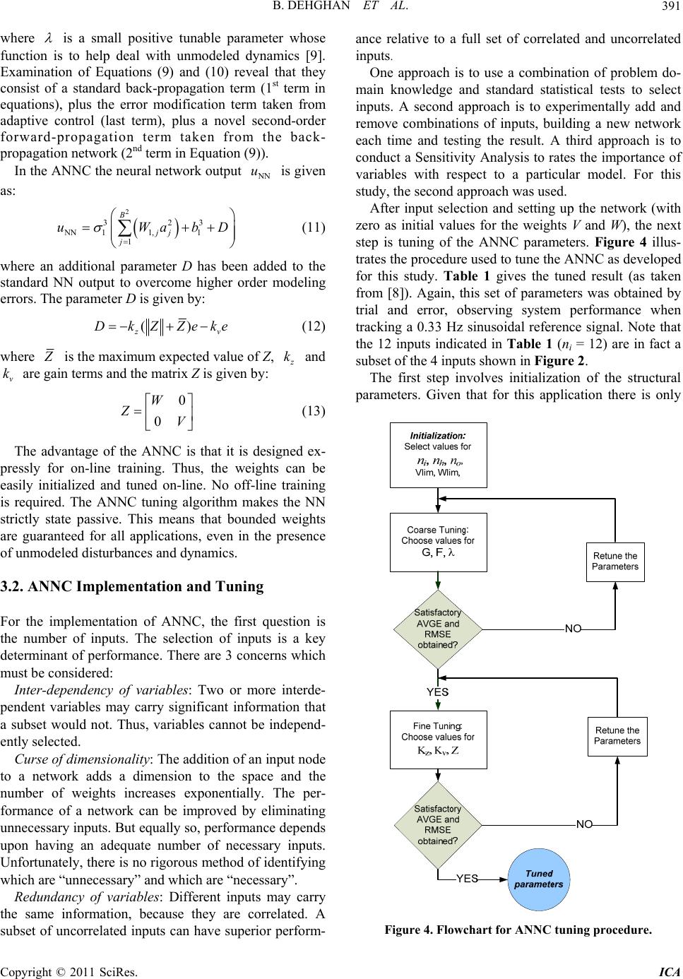
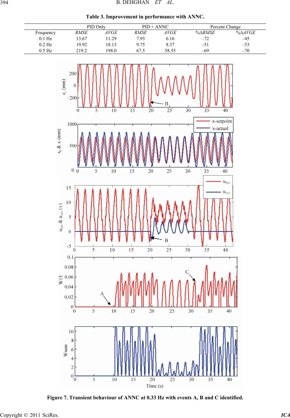
4.2. Transient Behaviour of ANNC
A series of additional tests were conducted at 0.33 Hz to
study the transient behaviour of ANNC and to confirm
that it was indeed “adapting”. Figure 7 illustrates system
response when the ANNC is turned on and off. There are
three events to highlight:
Event A (10 s)—ANNC learning starts (u = uPID)
Event B (20 s)—ANNC connected (u = uPID – uNN)
Event C (30 s)—ANNC disconnected (u = uPID)
The active adaptive nature of ANNC is clearly visible
and the result for this particular case is a 71% reduction
in AVGE. The weights reach their new values in just one
cycle. Note that Wsum is the sum of the elements of W and
thus exceeds the individual limit of 10 that seen in Table
1.
5. Conclusions
The potential of a novel adaptive on-line neural network
compensator (ANNC) for the position control of a
pneumatic gantry robot has been demonstrated. It was
found that by combining ANNC with a traditional PID
controller, tracking performance could be improved on
the order of 45% to 70%. This level of performance was
achieved after careful tuning of both the ANNC and PID
components. This paper documented the ANNC algo-
rithm and its tuning procedure, and presented experi-
mental results that illustrated the adaptive nature of NN
and confirmed the performance achievable with ANNC.
A major contribution is demonstration that tuning of
ANNC requires no more effort than the tuning of PID, in
that they both require the user to find values for only 3
parameters.
6. References
[1] G. M. Bone and S. Ning, “Experimental Comparison of
Position Tracking Control Algorithms for Pneumatic
Cylinder Actuators,” IEEE/ASME Transactions on Mecha-
tronics, Vol. 12, No. 5, 2007, pp. 557-561.
doi:10.1109/TMECH.2007.905718
[2] Y. Wang, H. Su, K. Harrington and G. Fischer, “Sliding
Mode Control of Piezoelectric Valve Regulated Pneu-
matic Actuator for MRI-Compatible Robotic Interven-
tion,” Proceeding of ASME Dynamic Systems and Con-
trol Conference, Cambridge, 12-15 September 2010, pp.
1-6.
[3] S. C. Gi, K. L. Han and H. C. Gi, “A Study on Tracking
Position Control of Pneumatic Actuators using Neural
Network,” Proceeding of 24th Annual Conference on IEEE
Industrial Electronics Society, Aachen, 31 Augudt-4 Sep-
tember 1998, pp. 1749-1753.
[4] D. C. Gross and K.S. Rattan, “Pneumatic Cylinder Tra-
jectory Tracking Control using a Feedforward Multilayer
Neural Network,” Proceedings of the IEEE 1997 Na-
tional Aerospace and Electronics Conference, Dayton,
14-17 July 1997, pp. 777-784.
doi:10.1109/NAECON.1997.622728
[5] Y. Li and T. Asakura, “A Study on Neural Network Con-
trol of Explosion-Proof 2-link Pneumatic Manipulator,”
2003 IEEE/ASME International Conference on Advanced
Intelligent Mechatronics, Kobe, 20-24 July 2003, pp.
1286-1291. doi:10.1109/AIM.2003.1225528
[6] X. Wang and G. Peng, “Modeling and Control for Pneu-
matic Manipulator Based on Dynamic Neural Network,”
Proceeding of IEEE International Conference on Systems,
Man and Cybernetics, Washington, DC, 5-8 October
2003, pp. 2231-2236.
[7] G. Kothapalli and M. Y. Hassan, “Design of a Neural
Network Based Intelligent PI Controller for a Pneumatic
System,” IAENG International Journal of Computer Sci-
ence, Vol. 35, No. 2, 2008, pp. 217-225.
[8] S. Taghizadeh, B. Surgenor and M. Abu Mallouh, “Con-
trol of a Pneumatic Gantry Robot with Adaptive Neural
Network Compensation,” Proceeding of 34th Mecha-
nisms and Robotics Conference, Montreal, 15-18 August
2010.
[9] F. L. Lewis, “Neural Network Control of Robot Manipu-
lators,” IEEE Expert, Vol. 11, No. 3, 1996, pp. 64-75.
doi:10.1109/64.506755
[10] G. Campa, M. Fravolini and M. Napolitano, “A Library
of Adaptive Neural Networks for Control Purposes,”
2002 IEEE International Symposium on Computer Aided
Control System Design, Glasgow, 18-20 September 2002,
pp. 115-120. doi:10.1109/CACSD.2002.1036939
[11] F. W. Lewis, S. Jagannathan and A. Yesildirak, “Neural
Network Control of Robot Manipulators and Non-Linear
Systems,” Taylor & Francis, London, 1999.
[12] R. C. Rice, “PID Tuning Guide,” Rockwell Automation,
Milwaukee, 2010.