Wireless Sensor Network, 2011, 3, 362-370
doi:10.4236/wsn.2011.311042 Published Online November 2011 (http://www.SciRP.org/journal/wsn)
A New Clustering Protocol for Wireless Sensor Networks
Using Genetic Algorithm Approach
Ali Norouzi1, Faezeh Sadat Babamir2, Abdul Halim Zaim3
1Department of Computer Engineering, Istanbul University/Avcilar, Istanbul, Turkey
2Department of Com p ut er Sci ence, Shahid Behesh ti University of Tehran, Tehran, Iran
3Department of Computer Engineering, Istanbul Commerce University/Eminonu, Istanbul, Turkey
Received October 2, 2011; revised October 21, 2011; accepted October 31, 2011
Abstract
This paper examines the optimization of the lifetime and energy consumption of Wireless Sensor Networks
(WSNs). These two competing objectives have a deep influence over the service qualification of networks
and according to recent studies, cluster formation is an appropriate solution for their achievement. To trans-
mit aggregated data to the Base Station (BS), logical nodes called Cluster Heads (CHs) are required to relay
data from the fixed-range sensing nodes located in the ground to high altitude aircraft. This study investi-
gates the Genetic Algorithm (GA) as a dynamic technique to find optimum states. It is a simple framework
that includes a proposed mathematical formula, which increasing in coverage is benchmarked against life-
time. Finally, the implementation of the proposed algorithm indicates a better efficiency compared to other
simulated works.
Keywords: Wireless Sensor Network, Energy Consumption, Genetic Algorithm, Cluster Based Fitness
Function
1. Introduction
Currently, sensor networks are employed in several areas,
including military, medical, environmental and house-
hold uses. But in all these fields, energy is the determi-
ning factor for the performance of wireless sensor net-
works [1]. Consequently, methods of data routing and
transfer to the base station are very important because the
sensor nodes run on battery power and the available e-
nergy for sensors is limited. A routing method with an
optimum consumption of energy and the shortest path
selection for data transfer in wireless sensor networks is
desired [2]. The main applications are for habitat mo-
nitoring, target tracking, surveillance and security [3,4].
A WSN consists of a number of small sensor nodes used
to entirely cover an environment; hence, the sensor nodes
should be low cost, low power and have limited energy
use. These nodes can communicate to each other across a
short distance. WSNs may be deployed either randomly
or deterministically, depending upon the application [5].
Deployment in a non-hazardous area is generally deter-
ministic while random placement is preferred in hazar-
dous or battlefield environments. In general, random
deployment requires more sensor nodes than determini-
stic deployment [6].
Generally, cluster based approaches are appropriate
for monitoring applications that require a continuous
stream of sensor data [3]; thus, routing protocols are ap-
plied to lower the cost of delivering a data packet on time.
For instance, Heinzelman et al. [7] study the LEACH
protocol, which is a hierarchical and self-organized clus-
ter-based approach. The area under monitoring is ran-
domly subdivided into several clusters in which CHs col-
lect data from the associated member nodes in their clu-
sters based on Time Division Multiple Access (TDMA)
scheduling. Then, redundant data is removed, and the
outcome is transmitted to the Base Station or sink as a
data packet. After a pre-determined period of time, CHs
are selected through a BS message.
Figure 1 shows a sample WSN with a series of red
circles surrounded by gray circles. The red circles re-
present a sensor/node, and the surrounding green circle is
the sensor detection range. There are several clusters that
transmit aggregated data to the BS just through CHs,
which are surrounded by gray circles. In this paper we
optimize the network life time and energy consumption in

363 A. NOROUZI ET AL.
Figure 1. A sample of cluster based WSN.
WSN and finally propose a new clustering protocol by
using genetic algorithm.
The remainder of this paper is arranged as follows: In
Section 2 we review the last works of clustering ap-
proach as literature.Section 3 is a brief description of GA
methodology concentrating on a WSN-based fitness fun-
ction. Our proposed intelligent technique of GA-based
clustering is presented in Section 4. Section 5 details the
simulation and implementation. Also results are dis-
cussed in Section 5 and finally, Section 6 presents our
conclusions and provides the direction of future projects.
2. Literature
Many studies are devoted to presenting algorithms in
which the costs, including receiving and transmitting
between CHs and BS, are reduced. Ghiasi et al. [8] pre-
sented theoretical work concentrating on the clustering
problem in WSN in order to optimize energy consump-
tion through optimal clustering of sensor nodes. Their
algorithm creates clusters with uniform size so that the
distance between sensor member nodes and CHs is
minimized; this minimization helps reduce the cost of
transmission energy [1,9].
Heinzelman et al. present a model for optimizing e-
nergy consumption, which is mentioned below. In this
formula, it is supposed that an energy node needs “ET
(i,
j)” energy to transmit “l” bit of data within a given dis-
tance of node i to node j.
,
4
2 ij
elij c
T
esij c
lEl ddd
ElEl ddd







o
o
(1)
“Ee” represents the amount of energy needed to acti-
vate electronic circuits for receiving and transmitting.
“dco” is the threshold value that “d4” is considered for
long distance and also “d2” for short rang transmission
such as within cluster [12]. Moreover, ""
s

=10 pJ/bit/m2
and ""
l

=0.0013 pJ/bit/m2 represent the energy con-
sumed by the amplifier for transmitting short and long
distances, respectively. Also, the required energy to re-
ceive l data bit is presumed to be Er = lEe in the receiver
In 2002, Lindsey et al. [10] proposed the PEGASIS
protocol, which was an extension of the LEACH algo-
rithm. The advantage of PEGASIS is in the robustness of
node failure compared to LEACH, while Pan et al. [11]
presented a two-tiered structure in which more energy
efficiency is provided by hierarchical clusters in certain
locations. Kalpakis et al. [12] proposed the MLDA
(Maximum Lifetime Data gathering Algorithm) to find
edge capacities that allow maximum transmission by
running a linear program. This algorithm is able to
maximize the lifetime of a network with certain locations
of each node and the BS. Dasgupta et al. [13] extended
MLDA by applying a cluster-based heuristic algorithm
called CMLDA, where nodes are grouped into several
pre-defined sized clusters. The energy summation of
cluster member nodes is their cluster’s energy. The dis-
tance between clusters is computed by the maximum
distance between every pair of nodes in two clusters.
After cluster formation, MLDA is applied. Bandyo-
padhyay et al. [14] proposed a multi-level hierarchical
clustering algorithm that utilizes stochastic geometry and
leads to minimized energy consumption. Cerpa et al. [15]
described the Adaptive Self-Configuring sensor Net-
works Topology (ASCENT), in which sensor nodes
manage their own connectivity, deciding whether to be
active and participate in multi-hop networking or to be
passive until receipt of a request from active nodes.
ASCENT can be used in any routing protocol in order to
handle node redundancy because it operates between link
layers and routing. In 2010, Jabari lotf et al. [16] pro-
posed an efficient cluster based algorithm named MLCH
to maximize lifetime. MLCH improves LEACH protocol
by using a very equally distributed cluster and also de-
creasing the unequal topology of clusters that clusters are
formed through radio range. It modifies the connection
distance of the head-nodes with cluster heads by hierar-
chical tree. An early example of a GA algorithm is Tur-
gut et al. work [17] which applied the GA concept to
improve mobile ad-hoc network clustering. The proposed
algorithm is the same as most of the GA based protocols
in that it presents a fitness parameter which defines the
destiny of an individual. Jin et al. [18] utilized GA to
reduce energy consumption. This algorithm determines a
primary number of pre-defined independently clustered
chromosomes and then biases them toward an optimal
solution with minimum communication distance. Simu-
lations have shown CH reduction by approximately 10%
of the total number of nodes. They also show that clus-
ter-based methods reduce 80% of the communication

A. NOROUZI ET AL.
364
distance, making it closer to the direct transmission dis-
tance. In 2005, Ferentinos et al. [19] improved the work
done by Jin et al. They investigated utilizing a fitness
function that involved the status of sensor nodes and
network clustering with suitable cluster heads, as well as
selecting between two signal ranges for normal sensor
nodes. Ye et al. [20] studied SMAC with a contention-
based medium access algorithm, in which a virtual clus-
ter agent reduces energy consumption. The researchers
also applied common sleep schedules for the clusters and
in-channel signaling in order to avoid collision.
In another direction, Hussian et al. [21,22] improved
the hierarchical cluster-based routing (HCR) protocol, in
which nodes self-cluster and are managed by the head set.
Of head set associates, a node is selected to head the
cluster and transmit monitored data based on the round
robin technique. Later, Hussain et al. [23] extended their
work using a genetic algorithm trick to obtain the opti-
mum number of clusters, cluster heads and cluster mem-
bers, as well as the transmission schedule. The proposed
fitness function is based on parameters such as energy
consumption, number of clusters, cluster size, direct dis-
tance to sink and cluster distance. In [3], they also worked
on an improvements to HCR (HCR-1) called HCR-2,
where they concluded that whenever more than 25% of
nodes have died, protocols including LEACH and HCR-1
tend to get disconnected quite rapidly while HCR-2 sur-
vives because of fewer elections. Whereas GA utilize
cross layer optimization, the energy consumption during
reconfiguration is minimal.
In 2011, Norouzi et al. [24] proposed a new protocol
called Fair Efficient Location-based Gossiping to address
the problems of Gossiping. We showed how our approach
increases the network energy and as a result maximizes
the network life time with using GA.
3. Genetic Al go ri t hm
A genetic algorithm is categorized as a global search
heuristic algorithm in which an optimal solution is esti-
mated by generating different individuals [24,25]. This
algorithm is comprised of procedures such as focused
fitness functions. Below, the fundamental parts of a ge-
netic algorithm are explained.
3.1. Initialization
Initially, the genetic algorithm begins with a primary
population including random chromosomes that consist
of genes with a sequence of 0 s or 1 s. In the next step,
the algorithm biases individuals toward the optimum
solution through repetitive processes such as crossover
and selection operators. A new population can be pro-
duced by two methods [26]: steady-state GA and genera-
tional GA. In the first case, one or two members of
population are replaced, while the generational GA re-
places all of the produced individuals at each generation.
In this paper, the second method is adopted so that the
GA keeps the specified qualified individuals from the
current generation and copies them into the new genera-
tion as part of the solution. Other individuals of the new
population are obtained by crossover and mutation func-
tions.
3.2. Fitness
The fitness function is defined for the genetic algorithm
as a scoring process to each chromosome according to
their qualifications. This value is a trait for survival and
further reproduction [26]. The fitness function is severely
problem dependent, so that for some problems, it is hard
or even impossible to define. In nature, individuals are
authorized to pass on to the new generation according to
their fitness value, which determines the fate of indi-
viduals.
3.3. Selection
During each successive generation, a new population is
generated by selecting members of the current generation
to mate based on fitness. Fitter individuals are almost
always selected, which leads to a preferential selection of
the best solution. Most of the functions have a stochasti-
cally designed element to choose small number of less fit
individuals to maintain the diversity of the population
[24]. Of the several selection methods, Roulette-Wheel is
chosen to distinguish appropriate individuals with the
following probability:
1
i
n
i
j
F
Pi
F



(2)
where Fi and ‘n’ are the fitness chromosome and the size
of population, respectively. According to the Roulette-
Wheel, each individual is assigned a value between 0 and
1.
3.4. Crossover
The main step for producing a new generation is the
crossover or reproduction process. In fact, it is a simula-
tion of the sexual reproductive process in that the inheri-
tance characteristics are naturally transferred into the
new population. To generate new children, crossover
process selects a pair of individuals as parents from the
collection determined by the breeding selection process.

A. NOROUZI ET AL. 365


This process will continue until the desired size of the
new population is obtained. In general, there are various
crossover operations that have been developed for diffe-
rent aims. The simplest method is single-point, in which
a random point is chosen to divide the contribution of the
two parents. Figure 2 shows an example of mating of
two chromosomes in single point way.
Figure 2 represents two children that from a single set
of parents. The bit sequence of the offspring duplicates
one parent’s bit sequence until the crossover point. After-
ward, the bit sequence of the other parent will be repli-
cated as the second part of children.
3.5. Fitness Parameters
The fitness of a chromosome represents its qualifications
on the bases of energy consumption minimization and
coverage maximization. Some important fitness parame-
ters are described below:
1) Direct Distance to Base Station (DDBS): total di-
rect distance between the whole sensor nodes and the BS,
denoted by di, is calculated as below:
1
m
i
i
DDBS d

 (3)
where ‘m’ is the number of nodes. As can be seen from
the above formula, energy consumption logically de-
pends on the number of nodes, such that it will be ex-
treme for large WSN. On the other hand, DDBS will be
acceptable for smaller networks with a few closely lo-
cated nodes.
2) Cluste r based Distance (CD): This parameter is the
sum of the distances between CHs and BS, added to the
sum of the distances between associated member nodes
and their cluster heads.
11
nm
ij is
ij
CDd D









 (4)
where ‘n’ and ‘m’ are the number of clusters and the
corresponding members, respectively. ‘dij’ is the distance
between a node and its CH, and ‘Dis’ is the distance be-
tween the CH and the BS. This solution is appropriate for
networks with a large number of widely-spaced
Parents Children
First: 10110101101101 01111010001011
 
Second: 10110110001011
01111001101101

Figure 2. Single point method at random point 6.
nodes. The cluster distance will be higher, which results
in higher energy consumption. In order to minimize en-
ergy consumption, the CD should not be too large [3].
Using this measurement, the density of the clusters will
be controlled, where density is the number of nodes per
cluster.
3) Cluster-based Distance-Standard Deviation (CDSD):
Standard derivation measures the variation of cluster
distances, rather than one average cluster distance.
CDSD is different depending on whether there is a ran-
dom or deterministic placement of sensor nodes. In the
case of random placement, there will be clusters of dif-
ferent sizes such that a SD within a specified variation in
the cluster distance is acceptable. In this case, the differ-
ences in cluster distance can be non-zero, but this varia-
tion should be adapted based on the deployment infor-
mation [6]. However, in deterministic placement where
node positions are uniformly distributed, the variation in
cluster distances should be small. In general, variation in
uniform cluster-based distances will indicate a poor net-
work, unlike a similar result when the nodes are ran-
domly placed.
In the following, µ computes the average of the cluster
distances, which will be our standard SD formula for
computing cluster distance variation.
1
n
c
i
d
n




(5)

2
1
n
c
i
SD d 


 (6)
4) Transfer Energy (E): This metric, E, indicates the
amount of consumed energy to transfer all the collected
data to the BS. Considering m-many associated nodes in
a cluster, E is computed as follows:
11
*
nm
j
mR
ij
EemE





 i
e (7)
where ejm is the energy necessary to transmit data from a
node to the corresponding CH. Therefore, the first term
in the summation of ‘i’ is the total energy consumed in
transferring the aggregated data to CHs. The second term
in the ‘i’ summation shows the energy required to re-
ceive data from members, and finally ei represents the
energy needed to transmit from the cluster head to the
BS.
5) Number of Transmissions (T): Generally, the BS
determines number of transmissions for each monitoring
period. This measure is computed according to the con-
ditions and the energy level of the network; consequently,
a large T represents a long time stage for which only a
superior optimum solution for maximization and an infe-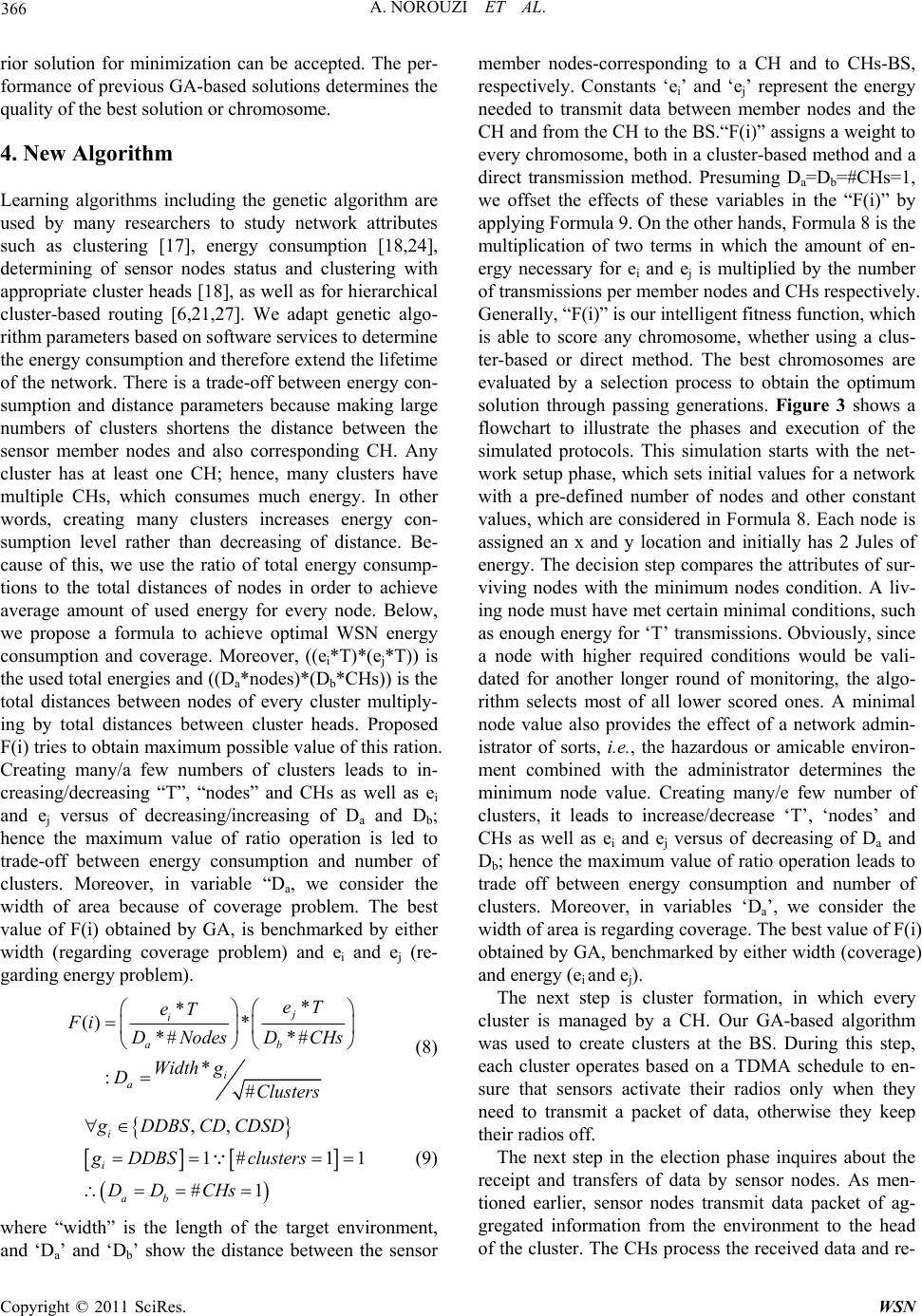

A. NOROUZI ET AL.
366
rior solution for minimization can be accepted. The per-
formance of previous GA-based solutions determines the
quality of the best solution or chromosome.
4. New Algorithm
Learning algorithms including the genetic algorithm are
used by many researchers to study network attributes
such as clustering [17], energy consumption [18,24],
determining of sensor nodes status and clustering with
appropriate cluster heads [18], as well as for hierarchical
cluster-based routing [6,21,27]. We adapt genetic algo-
rithm parameters based on software services to determine
the energy consumption and therefore extend the lifetime
of the network. There is a trade-off between energy con-
sumption and distance parameters because making large
numbers of clusters shortens the distance between the
sensor member nodes and also corresponding CH. Any
cluster has at least one CH; hence, many clusters have
multiple CHs, which consumes much energy. In other
words, creating many clusters increases energy con-
sumption level rather than decreasing of distance. Be-
cause of this, we use the ratio of total energy consump-
tions to the total distances of nodes in order to achieve
average amount of used energy for every node. Below,
we propose a formula to achieve optimal WSN energy
consumption and coverage. Moreover, ((ei*T)*(ej*T)) is
the used total energies and ((Da*nodes)*(Db*CHs)) is the
total distances between nodes of every cluster multiply-
ing by total distances between cluster heads. Proposed
F(i) tries to obtain maximum possible value of this ration.
Creating many/a few numbers of clusters leads to in-
creasing/decreasing “T”, “nodes” and CHs as well as ei
and ej versus of decreasing/increasing of Da and Db;
hence the maximum value of ratio operation is led to
trade-off between energy consumption and number of
clusters. Moreover, in variable “Da, we consider the
width of area because of coverage problem. The best
value of F(i) obtained by GA, is benchmarked by either
width (regarding coverage problem) and ei and ej (re-
garding energy problem).
*
*
() *
*# *#
*
:#
j
i
ab
i
a
eT
eT
Fi DNodesDCHs
Width g
DClusters









(8)

 

,,
1# 11
#1
i
i
ab
gDDBSCD CDSD
g DDBSclusters
DD CHs

 
 
 (9)
where “width” is the length of the target environment,
and ‘Da’ and ‘Db’ show the distance between the sensor
member nodes-corresponding to a CH and to CHs-BS,
respectively. Constants ‘ei’ and ‘ej’ represent the energy
needed to transmit data between member nodes and the
CH and from the CH to the BS.“F(i)” assigns a weight to
every chromosome, both in a cluster-based method and a
direct transmission method. Presuming Da=Db=#CHs=1,
we offset the effects of these variables in the “F(i)” by
applying Formula 9. On the other hands, Formula 8 is the
multiplication of two terms in which the amount of en-
ergy necessary for ei and ej is multiplied by the number
of transmissions per member nodes and CHs respectively.
Generally, “F(i)” is our intelligent fitness function, which
is able to score any chromosome, whether using a clus-
ter-based or direct method. The best chromosomes are
evaluated by a selection process to obtain the optimum
solution through passing generations. Figure 3 shows a
flowchart to illustrate the phases and execution of the
simulated protocols. This simulation starts with the net-
work setup phase, which sets initial values for a network
with a pre-defined number of nodes and other constant
values, which are considered in Formula 8. Each node is
assigned an x and y location and initially has 2 Jules of
energy. The decision step compares the attributes of sur-
viving nodes with the minimum nodes condition. A liv-
ing node must have met certain minimal conditions, such
as enough energy for ‘T’ transmissions. Obviously, since
a node with higher required conditions would be vali-
dated for another longer round of monitoring, the algo-
rithm selects most of all lower scored ones. A minimal
node value also provides the effect of a network admin-
istrator of sorts, i.e., the hazardous or amicable environ-
ment combined with the administrator determines the
minimum node value. Creating many/e few number of
clusters, it leads to increase/decrease ‘T’, ‘nodes’ and
CHs as well as ei and ej versus of decreasing of Da and
Db; hence the maximum value of ratio operation leads to
trade off between energy consumption and number of
clusters. Moreover, in variables ‘Da’, we consider the
width of area is regarding coverage. The best value of F(i)
obtained by GA, benchmarked by either width (coverage)
and energy (ei and ej).
The next step is cluster formation, in which every
cluster is managed by a CH. Our GA-based algorithm
was used to create clusters at the BS. During this step,
each cluster operates based on a TDMA schedule to en-
sure that sensors activate their radios only when they
need to transmit a packet of data, otherwise they keep
their radios off.
The next step in the election phase inquires about the
receipt and transfers of data by sensor nodes. As men-
tioned earlier, sensor nodes transmit data packet of ag-
gregated information from the environment to the head
of the cluster. The CHs process the received data and re-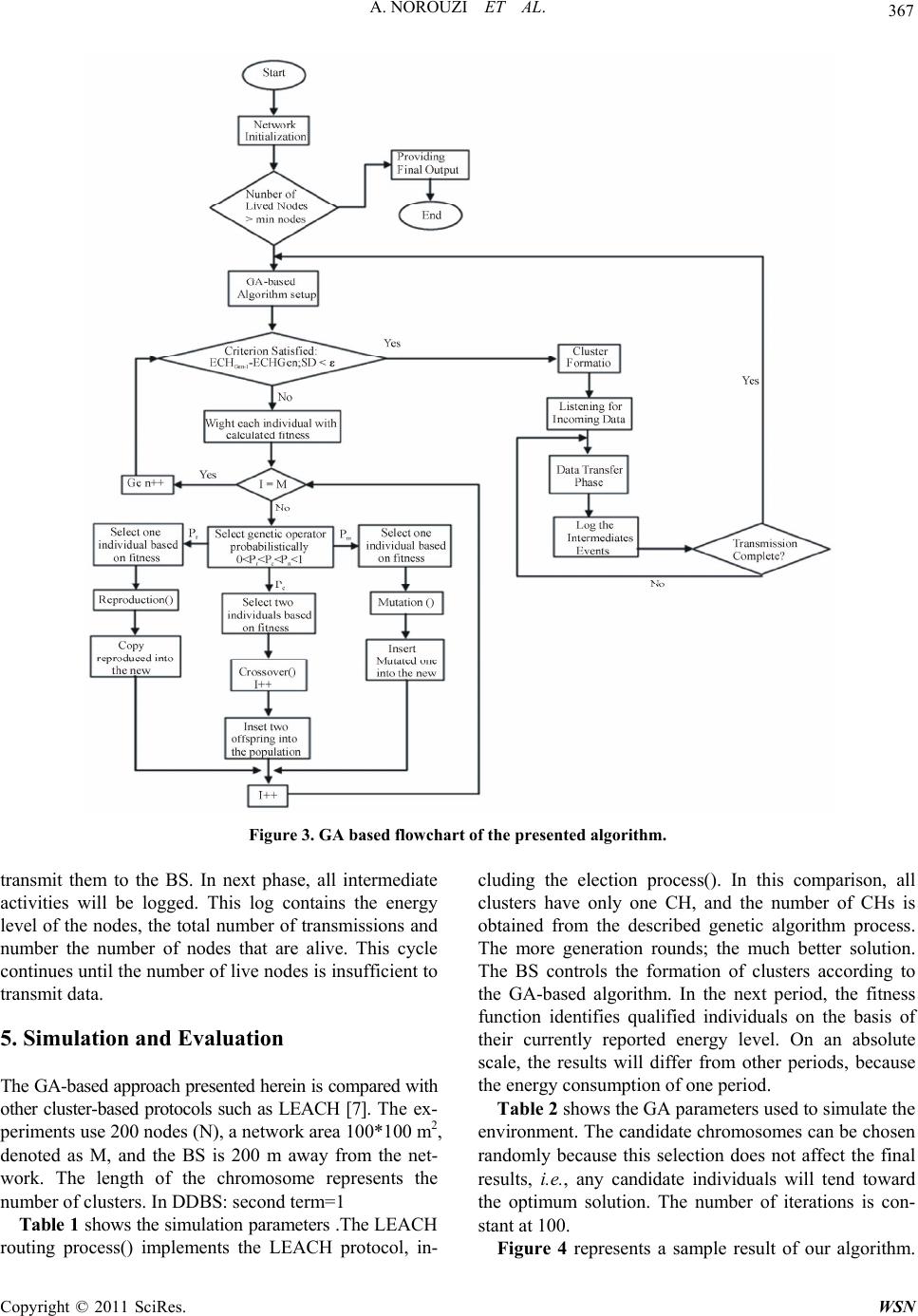

A. NOROUZI ET AL.
367
Figure 3. GA based flowchart of the presented algorithm.
transmit them to the BS. In next phase, all intermediate
activities will be logged. This log contains the energy
level of the nodes, the total number of transmissions and
number the number of nodes that are alive. This cycle
continues until the number of live nodes is insufficient to
transmit data.
5. Simulation and Evaluation
The GA-based approach presented herein is compared with
other cluster-based protocols such as LEACH [7]. The ex-
periments use 200 nodes (N), a network area 100*100 m2,
denoted as M, and the BS is 200 m away from the net-
work. The length of the chromosome represents the
number of clusters. In DDBS: second term=1
Table 1 shows the simulation parameters .The LEACH
routing process() implements the LEACH protocol, in-
cluding the election process(). In this comparison, all
clusters have only one CH, and the number of CHs is
obtained from the described genetic algorithm process.
The more generation rounds; the much better solution.
The BS controls the formation of clusters according to
the GA-based algorithm. In the next period, the fitness
function identifies qualified individuals on the basis of
their currently reported energy level. On an absolute
scale, the results will differ from other periods, because
the energy consumption of one period.
Table 2 shows the GA parameters used to simulate the
environment. The candidate chromosomes can be chosen
randomly because this selection does not affect the final
results, i.e., any candidate individuals will tend toward
the optimum solution. The number of iterations is con-
stant at 100.
Figure 4 represents a sample result of our algorithm.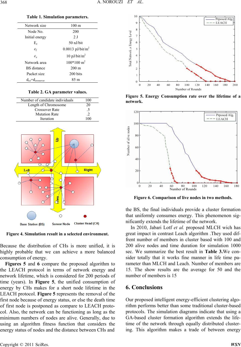

A. NOROUZI ET AL.
368
Table 1. Simulation parameters.
Network size 100 m
Node No. 200
Initial energy 2 J
Ee 50 nJ/bit
l

0.0013pJ/bit/m2
s

10 pJ/bit/m2
Network area 100*100 m2
BS distance 200 m
Packet size 200 bits
dco=dcrossove r 85 m
Table 2. GA parameter values.
Number of candidate individuals 100
Length of Chromosome 20
Crossover Rate .5
Mutation Rate .2
Iteration 100
Figure 4. Simulation result in a selected environment.
Because the distribution of CHs is more unified, it is
highly probable that we can achieve a more balanced
consumption of energy.
Figures 5 and 6 compare the proposed algorithm to
the LEACH protocol in terms of network energy and
network lifetime, which is considered for 200 periods of
time (years). In Figure 5, the unified consumption of
energy by CHs makes for a short node lifetime in the
LEACH protocol. Figure 5 represents the removal of the
first node because of energy status, or else the death time
of first node is postponed as compare to LEACH proto-
col. Also, the network can be functioning as long as the
minimum numbers of nodes are alive. Generally, due to
using an algorithm fitness function that considers the
energy status of nodes and the distance between CHs and
Figure 5. Energy Consumption rate over the lifetime of a
network.
Number of Rounds
Figure 6. Comparison of live nodes in two methods.
the BS, the final individuals provide a cluster formation
that uniformly consumes energy. This phenomenon sig-
nificantly extends the lifetime of the network.
In 2010, Jabari Lotf et al. proposed MLCH wich has
great impact in contrast Leach algorithm .They used dif-
frent number of members in cluster based with 100 and
200 alive nodes and time duration for simulation 1000
sec. We summarize the best result in Table 3.We con-
sider totally that it works fine manner in life time pa-
rameter than MLCH and Leach. Number of members are
15. The show results are the average for 50 and the
number of members is 15
6. Conclusions
Our proposed intelligent energy-efficient clustering algo-
rithm performs better than some traditional cluster-based
protocols. The simulation diagrams indicate that using a
GA-based cluster formation algorithm extends the life-
time of the network through equally distributed cluster-
ing. This algorithm makes a trade of between energy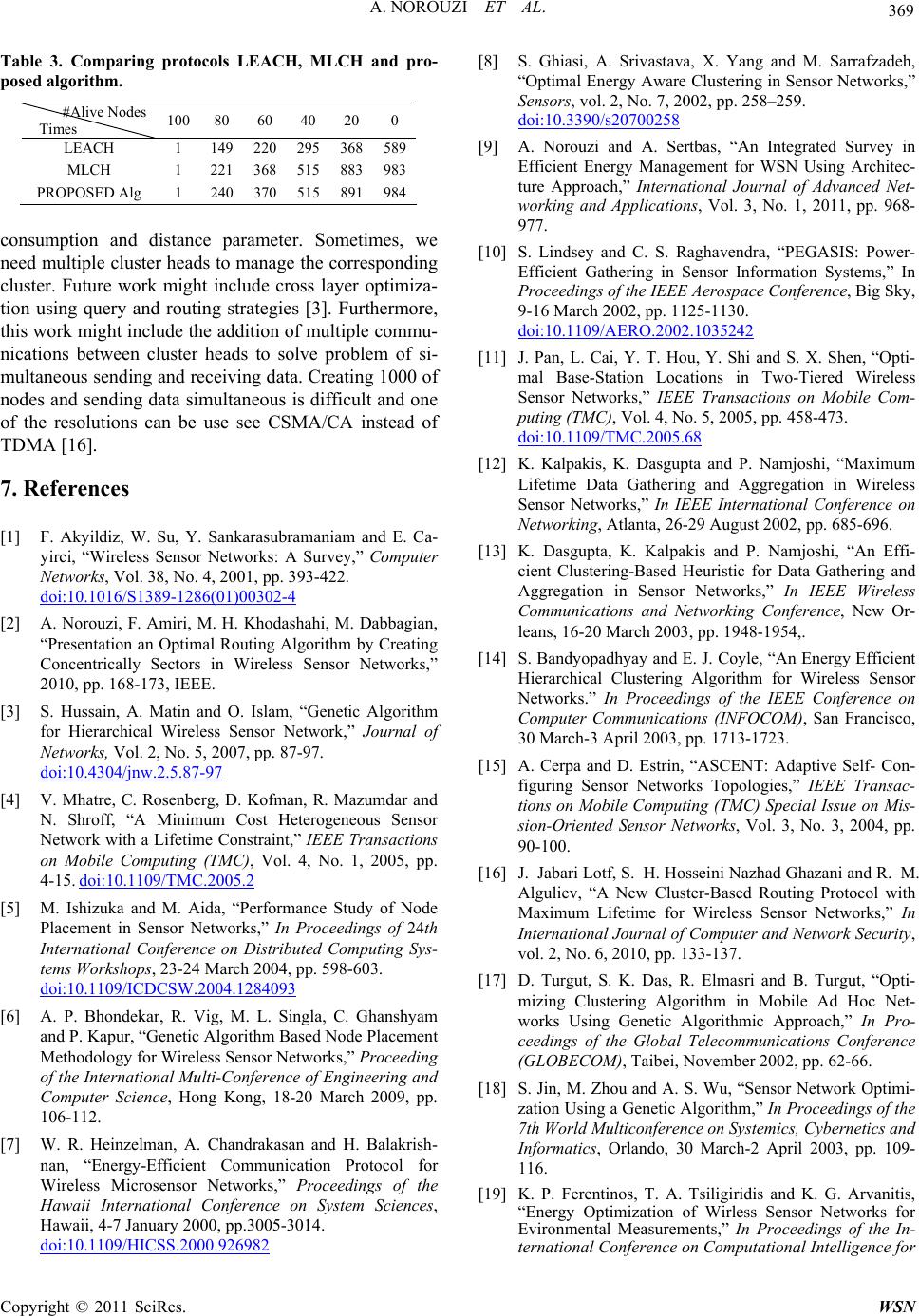

369 A. NOROUZI ET AL.
Table 3. Comparing protocols LEACH, MLCH and pro-
posed algorithm.
#Alive Nodes
Times 100 80 60 40 20 0
LEACH 1 149 220 295 368589
MLCH 1 221 368 515 883983
PROPOSED Alg 1 240 370 515 891 984
consumption and distance parameter. Sometimes, we
need multiple cluster heads to manage the corresponding
cluster. Future work might include cross layer optimiza-
tion using query and routing strategies [3]. Furthermore,
this work might include the addition of multiple commu-
nications between cluster heads to solve problem of si-
multaneous sending and receiving data. Creating 1000 of
nodes and sending data simultaneous is difficult and one
of the resolutions can be use see CSMA/CA instead of
TDMA [16].
7. References
[1] F. Akyildiz, W. Su, Y. Sankarasubramaniam and E. Ca-
yirci, “Wireless Sensor Networks: A Survey,” Computer
Networks, Vol. 38, No. 4, 2001, pp. 393-422.
doi:10.1016/S1389-1286(01)00302-4
[2] A. Norouzi, F. Amiri, M. H. Khodashahi, M. Dabbagian,
“Presentation an Optimal Routing Algorithm by Creating
Concentrically Sectors in Wireless Sensor Networks,”
2010, pp. 168-173, IEEE.
[3] S. Hussain, A. Matin and O. Islam, “Genetic Algorithm
for Hierarchical Wireless Sensor Network,” Journal of
Networks, Vol. 2, No. 5, 2007, pp. 87-97.
doi:10.4304/jnw.2.5.87-97
[4] V. Mhatre, C. Rosenberg, D. Kofman, R. Mazumdar and
N. Shroff, “A Minimum Cost Heterogeneous Sensor
Network with a Lifetime Constraint,” IEEE Transactions
on Mobile Computing (TMC), Vol. 4, No. 1, 2005, pp.
4-15. doi:10.1109/TMC.2005.2
[5] M. Ishizuka and M. Aida, “Performance Study of Node
Placement in Sensor Networks,” In Proceedings of 24th
International Conference on Distributed Computing Sys-
tems Workshops, 23-24 March 2004, pp. 598-603.
doi:10.1109/ICDCSW.2004.1284093
[6] A. P. Bhondekar, R. Vig, M. L. Singla, C. Ghanshyam
and P. Kapur, “Genetic Algorithm Based Node Placement
Methodology for Wireless Sensor Networks,” Proceeding
of the International Multi-Conference of Engineering and
Computer Science, Hong Kong, 18-20 March 2009, pp.
106-112.
[7] W. R. Heinzelman, A. Chandrakasan and H. Balakrish-
nan, “Energy-Efficient Communication Protocol for
Wireless Microsensor Networks,” Proceedings of the
Hawaii International Conference on System Sciences,
Hawaii, 4-7 January 2000, pp.3005-3014.
doi:10.1109/HICSS.2000.926982
[8] S. Ghiasi, A. Srivastava, X. Yang and M. Sarrafzadeh,
“Optimal Energy Aware Clustering in Sensor Networks,”
Sensors, vol. 2, No. 7, 2002, pp. 258–259.
doi:10.3390/s20700258
[9] A. Norouzi and A. Sertbas, “An Integrated Survey in
Efficient Energy Management for WSN Using Architec-
ture Approach,” International Journal of Advanced Net-
working and Applications, Vol. 3, No. 1, 2011, pp. 968-
977.
[10] S. Lindsey and C. S. Raghavendra, “PEGASIS: Power-
Efficient Gathering in Sensor Information Systems,” In
Proceedings of the IEEE Aerospace Conference, Big Sky,
9-16 March 2002, pp. 1125-1130.
doi:10.1109/AERO.2002.1035242
[11] J. Pan, L. Cai, Y. T. Hou, Y. Shi and S. X. Shen, “Opti-
mal Base-Station Locations in Two-Tiered Wireless
Sensor Networks,” IEEE Transactions on Mobile Com-
puting (TMC), Vol. 4, No. 5, 2005, pp. 458-473.
doi:10.1109/TMC.2005.68
[12] K. Kalpakis, K. Dasgupta and P. Namjoshi, “Maximum
Lifetime Data Gathering and Aggregation in Wireless
Sensor Networks,” In IEEE International Conference on
Networking, Atlanta, 26-29 August 2002, pp. 685-696.
[13] K. Dasgupta, K. Kalpakis and P. Namjoshi, “An Effi-
cient Clustering-Based Heuristic for Data Gathering and
Aggregation in Sensor Networks,” In IEEE Wireless
Communications and Networking Conference, New Or-
leans, 16-20 March 2003, pp. 1948-1954,.
[14] S. Bandyopadhyay and E. J. Coyle, “An Energy Efficient
Hierarchical Clustering Algorithm for Wireless Sensor
Networks.” In Proceedings of the IEEE Conference on
Computer Communications (INFOCOM), San Francisco,
30 March-3 April 2003, pp. 1713-1723.
[15] A. Cerpa and D. Estrin, “ASCENT: Adaptive Self- Con-
figuring Sensor Networks Topologies,” IEEE Transac-
tions on Mobile Computing (TMC) Special Issue on Mis-
sion-Oriented Sensor Networks, Vol. 3, No. 3, 2004, pp.
90-100.
[16] J. Jabari Lotf, S. H. Hosseini Nazhad Ghazani and R. M.
Alguliev, “A New Cluster-Based Routing Protocol with
Maximum Lifetime for Wireless Sensor Networks,” In
International Journal of Computer and Network Security,
vol. 2, No. 6, 2010, pp. 133-137.
[17] D. Turgut, S. K. Das, R. Elmasri and B. Turgut, “Opti-
mizing Clustering Algorithm in Mobile Ad Hoc Net-
works Using Genetic Algorithmic Approach,” In Pro-
ceedings of the Global Telecommunications Conference
(GLOBECOM), Taibei, November 2002, pp. 62-66.
[18] S. Jin, M. Zhou and A. S. Wu, “Sensor Network Optimi-
zation Using a Genetic Algorithm,” In Proceedings of the
7th World Multiconference on Systemics, Cybernetics and
Informatics, Orlando, 30 March-2 April 2003, pp. 109-
116.
[19] K. P. Ferentinos, T. A. Tsiligiridis and K. G. Arvanitis,
“Energy Optimization of Wirless Sensor Networks for
Evironmental Measurements,” In Proceedings of the In-
ternational Conference on Computational Intelligence for

A. NOROUZI ET AL.
370
Measurment Systems and Applicatons (CIMSA), La Co-
runa, 10-12 July 2005, pp. 1031-1051.
[20] W. Ye, J. Heidemann and D. Estrin, “Medium Access
Control with Coordinated Adaptive Sleeping for Wireless
Sensor Networks,” IEEE/ACM Transactions on Networks,
Vol. 12, No. 3, 2004, pp. 493–506.
doi:10.1109/TNET.2004.828953
[21] S. Hussain and A. W. Matin, “Base Station Assisted Hi-
erarchical Cluster-Based Routing,” In IEEE/ACM Inter-
national Conference on Wireless and Mobile communica-
tions Network (ICWMC), Bucharest, 29-31 July 2006, p.
9.
[22] A. W. Matin and S. Hussain, “Intelligent Hierarchical
Cluster-Based Routing,” In International Workshop on
Mobility and Scalability in Wireless Sensor Networks
(MSWSN), CTI Press, Athens, 2006, pp. 165-172.
[23] S. Hussain, A. W. Matin and O. Islam, “Genetic Algo-
rithm for Energy Efficient Clusters in Wireless Sensor
Networks,” In Fourth International Conference on In-
formation Technology: New Generations (ITNG 2007),
Las Vegas, 2-4, April 2007, pp.147-154.
[24] A.Norouzi, F.S Babamir and A.H.Zaim, “A Novel
Energy Efficient Routing Protocol in Wireless Sensor
Networks,” Journal of Wireless Sensor Network, Vol. 3
No. 10, 2011, pp. 1-10.
[25] D. E. Goldberg, “Genetic Algorithm in a Search Optimi-
zation and Machine Learning,” Addison Wesley, Boston,
1989, pp. 191-206.
[26] V. Kreinovich, C. Quintana and O. Fuentes, “Genetic
Algorithms―What Fitness Scaling is Optimal?” Cyber-
netics and Systems: An International Journal, Vol. 24, No.
1, 1933, pp. 9-26.
[27] A. W. Matin and S. Hussain, “Intelligent Hierarchical
Cluster-Based Routing,” In International Workshop on
Mobility and Scalability in Wireless Sensor Networks
(MSWSN), CTI Press, Athens, 2006, pp. 165-172.
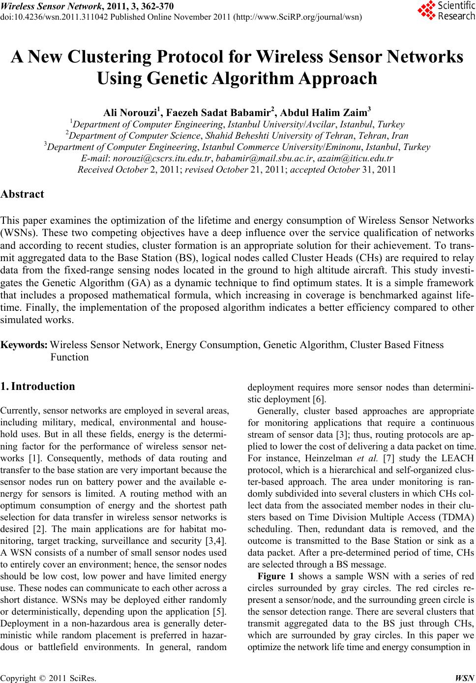