Journal of Applied Mathematics and Physics
Vol.06 No.01(2018), Article ID:82288,10 pages
10.4236/jamp.2018.61030
Hölder Regularity for Abstract Fractional Cauchy Problems with Order in (0,1)
Chenyu Li, Miao Li
Department of Mathematics, Sichuan University, Chengdu, China


Received: August 30, 2017; Accepted: January 28, 2018; Published: January 31, 2018
ABSTRACT
In this paper, we study the regularity of mild solution for the following fractional abstract Cauchy problem on a Banach space X with order , where the fractional derivative is understood in the sense of Caputo fractional derivatives. We show that if A generates an analytic α-times resolvent family on X and for some , then the mild solution to the above equation is in for every . Moreover, if f is Hölder continuous, then so are the and .
Keywords:
Fractional Cauchy Problem, Fractional Resolvent Family, Generator, Regularity, Hölder Continuity

1. Introduction
Recently there are increasing interests on fractional differential equations due to their wide applications in viscoelasticity, dynamics of particles, economic and science et al. For more details we refer to [1] [2].
Many evolution equations can be rewritten as an abstract Cauchy problem, and then they can be studied in an unified way. For example, a heat equation with different initial data or boundary conditions can be written as a first order Cauchy problem, in which the governing operator generates a C0-semigroup, and then the solution is given by the operation of this semigroup on the initial data. See for instance [3] [4]. Prüss [5] developed the theory of solution operators to research some abstract Volterra integral equations and it was Bajlekova [6] who first use solution operators to discuss the fractional abstract Cauchy problems. If the coefficient operator of a fractional abstract Cauchy problem generates a C0-semigroup, we can invoke an operator described by the C0-semigroup and a probability density function to solve this problem, for more details we refer to [7] [8] [9]. The vector-valued Laplace transform developed in [3] is an important tool in the theory of fractional differential equations.
There are some papers devoted to the fractional differential equations in many different respects: the connection between solutions of fractional Cauchy problems and Cauchy problems of first order [10]; the existence of solution of several kinds of fractional equations [11] [12]; the Hölder regularity for a class of fractional equations [13] [14]; the maximal regularity for fractional order equations [6]; the boundary regularity for the fractional heat equation [15]; the relation of continuous regularity for fractional order equations with semi-variations [12]. In this paper we are mainly interested in the Hölder regularity for abstract Cauchy problems of fractional order.
Pazy [4] considered the regularity for the abstract Cauchy problem of first order:
(1.1)
where A is the infinitesimal generator of an analytic C0-semigroup. He showed that if for some , then is Hölder continuous with
exponent in ; if moreover , then u is Hölder continuous
with the same exponent in . If in addition f is Hölder continuous, then
Pazy showed that there are some further regularity of and . Li [16]
gave similar results for fractional differential equations with order . In this paper we will extend their results to fractional Cauchy problems with order in .
Our paper is organized as follows. In Section 2 there are some preliminaries on fractional derivatives, fractional Cauchy problems and fractional resolvent families. In Section 3 we give the regularity of the mild solution under the condition that . And some further continuity results are given in Section 4.
2. Preliminaries
Let A be a closed densely defined linear operator on a Banach space X. In this paper we consider the following equation:
(2.1)
where u and f are X-valued functions, , and is the Caputo fractional derivative defined by
in which for ,
and is understood as the Dirac measure at 0. The convolution of two functions f and g is defined by
when the above integrals exist.
The classical (or strong) solution to (2.1) is defined as:
Definition 2.1. If , is called a solution of (2.1) if
1) .
2) .
3) u satisfies (2.1) on .
By integration (2.1) for α-times, we are able to define a kind of weak solutions.
Definition 2.2. If , is called a mild solution of (2.1) if for every and
And it is therefore natural to give the following definition of α-resolvent family for the operator A.
Definition 2.3. A family is called an α-resolvent family for the operator A if the following conditions are satisfied:
1) is continuous for every and ;
2) and for all and ;
3) the resolvent equation
holds for every .
If there is an α-times resolvent family for the operator A, then the mild solution of (2.1) is given by the following lemma.
Lemma 2.4. [10] Let A generate an α-times resolvent family and let . If (2.1) has a mild solution, then it is given by
For the strong solution of (2.1), we have
Lemma 2.5. [10] Let A generate an α-times resolvent family and let , . If , then the following statements are equivalent:
(a) (2.1) has a strong solution on .
(b) is differentiable on .
(c) for and is
continuous on .
If in addition, the α-times resolvent family admits an analytic extension to some sector , and for all , we will then denote it by .
If , then there exists constants C, and such that and
(2.2)
for each . The α-times resolvent family generated by A can be given by
where
is oriented counter-clockwise. And the corresponding operators are defined by
Lemma 2.6. Let and . We have
(1) for every and for ;
(2) for every , and for ;
(3) for , for any integer and for , where .
Proof. (1) By the definition of and (2.2),
Since
taking , we can obtain that the above integral is bounded by
Analogously one can show the estimate
It thus follows the estimate for .
(2) By the identity , we have
since . Moreover,
By the closedness of the operator A, the assertion of (2) follows.
(3) By the proof of (2) and the closedness of A,
And the second part of (3) can be proved similarly. □
Remark 2.7. Similar results for were given in [16]. It is obvious that
if and
if .
3. Regularity of the Mild Solutions
In this section we consider the mild solution of (2.1) with . Suppose that the operator A generates an analytic α-resolvent family, then by Lemma 2.4 and Remark 2.7 the mild solution of (2.1) is given by
(3.1)
Theorem 3.1. Let , , and with .
Then for every and , , where is given
by (3.1). If moreover such that , then .
Proof. Since is analytic, we only need to show that .
Let and , then
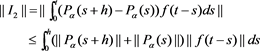
By Hölder’s inequality and Lemma 2.6,
We remark that the constant C here and in the sequel may be vary line by line, but not depending on t and h. Next, we estimate . For , , first assume that ,
since ; if
; if , then
from which it follows also that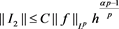 .
.
If  with
with , then by [[10], Lemma 4.5] we have that
  is differentiable and thus Lipschitz continuous. □
If we put more conditions on , the regularity of
  can be raised.
Proposition 3.2. Let ,
,  and
and  with
with . For every
 , we define the function
  by
by
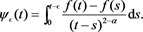
If 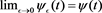 exists, then for every
 ,
, . If moreover
 , then
 .
.
Proof. If  satisfies the assumption, by [[17], Theorem 13.2] there exists a function
  such that
 . Thus

Since  is analytic and bounded,
 . It is easy to see
that  is Hölder continuous with index
 . This completes the
proof. □
4. Regularity of the Classical Solutions
Motivated by the results in [18] for the C0-semigroups, we first give the following proposition.
Proposition 4.1. Let  and
and . Assume
 ,
,  and
and . Then the mild solution of (2.1) is the classical solution.
Proof. By Lemma 2.5 we only need to show that  for every
  and
and  is continuous on
 . We decompose
  into two parts:

where

belongs to  and is continuous. To prove that
 , we define the following functions:

and

for  small enough. It is clear that
  as
as . Moreover.

for all , it follows from the fact that for a fix
  the map
  is a continuous mapping, we conclude that

By our assumption and Lemma 2.6 there exists a constant  such that

consequently, the function  is integrable. Hence by the closedness of A we obtain that

The continuity of the function  follows directly from the fact

This completes the proof. □
We will then give the regularity of such classical solutions.
Lemma 4.2. Let  with
with , and
, and  with
with . Define

Then for any ,
,  and
and .
.
Proof. For fixed , since
  we have

By the closedness of A, we obtain . Thus it remains to show that
 . For
. For  and
and  we have the following decomposition:

Since  we have

We can estimate  as follows:

And it is easy to show that . Combining all above we have
 . □
. □
The following theorem extends [[16], Theorem 4.4] to the case that .
.
Theorem 4.3. Let  with
with ,
,  with
with ,
,  , and u is the classical solution of (2.1). The following assertions hold.
(1) For every ,
,  ,
, .
.
(2) If moreover , then
  and
and  are continuous on
 .
.
(3) If , then
  and
and .
.
Proof. (1) If u is the classical solution of (2.1) on , then
 . It is only need to prove
  We decompose

By Lemma 4.2, . Let
. Let . If
. If , then


thus we have

(2) We only need to show that  is continuous at
 . Since
  and
and  is continuous,

as .
.
(3) We show that . Indeed, this follows from

5. Conclusion
In this paper, we proved the Hölder regularity of the mild and strong solutions to the α-order abstract Cauchy problem (2.1) with . Our results are complemental to the existing results of Pazy [18] for the case
  and Li [16] for the case that
 .
.
Cite this paper
Li, C.Y. and Li, M. (2018) Hölder Regularity for Abstract Fractional Cauchy Problems with Order in (0,1). Journal of Applied Mathematics and Physics, 6, 310-319. https://doi.org/10.4236/jamp.2018.61030
References
- 1. Hilfer, R. (2000) Applications of Fractional Calculus in Physics. World Scientific, Singapore.
- 2. Tarasov, V. (2011) Fractional Dynamics: Applications of Fractional Calculus to Dynamics of Particles, Fields and Media. Springer, New York.
- 3. Arendt, W., Batty, C.J.K., Hieber, M. and Neubrander, F. (2010) Vector-Valued Laplace Transforms and Cauchy Problems. Birkhäuser,.
- 4. Pazy, A. (1983) Semigroups of Linear Operators and Applications to Partial Differential Equations. Springer, New York.
- 5. Prüss, J. (1993) Evolutionary Integral Equations and Applications. Birkhäuser, Basel.
- 6. Bajlekova, E.G. (2001) Fractional Evolution Equations in Banach Spaces. Ph.D. Thesis, Department of Mathematics, Eindhoven University of Technology.
- 7. EI-Boral, M.M. (2004) Semi-group and Some Nonlinear Fractional Differential Equations. Appl. Math. Comput., 149, 823-831.
- 8. EI-Boral, M.M. (2002) Some Probability Densities and Fundamental Solutions of Fractional Evolution Equations. Chaos Solitons Fractals, 14, 433-440. https://doi.org/10.1016/S0960-0779(01)00208-9
- 9. EI-Boral, M.M., EI-Nadi, K.E. and EI-Akabawy, E.G. (2010) On Some Fractional Evolution Equations. Comput. Math. Anal., 59, 1352-1355.
- 10. Li, M., Chen, C. and Li, F.B. (2010) On Fractional Powers of Generators of Fractional Resolvent Families. J. Funct. Anal., 259, 2702-2726.
- 11. Akrami, M.H. and Erjaee, G.H. (2014) Existence of Positive Solutions for a Class of Fractional Differential Equation Systems with Multi-Point Boundary Conditions. Georgian Math. J., 21, 379-386.
- 12. Li, F.B. and Li, M. (2013) On Maximal Regularity and Semivariation of Times Resolvent Families. Pure Math., 3, 680-684.
- 13. Clément, P., Gripenberg, G. and Londen, S-O. (2000) Schauder Estimates for Equations with Fractional Derivatives. Trans. Amer. Math. Soc., 352, 2239-2260.
- 14. Clément, P., Gripenberg, G. and Londen, S-O. (1998) Hölder Regularity for a Linear Fractional Evolution Equations, Topics in Nonlinear Analysis. The Herbert Amann Anniversary Volume, Birkhäuser, Basel.
- 15. Fernandez-Real, X. and Ros-Oton, X. (2016) Boundary Regularity for the Fractional Heat Equation, RACSAM110.
- 16. Li, Y. (2015) Regularity of Mild Solutions for Fractional Abstract Cauchy Problem with Order , Z. Angew. Math. Phys., 66, 3283-3298.
- 17. Samko, S.G., Klibas, A.A. and Marichev, O.I. (1992) Fractional Integrals and Derivatives, Theory and Applications. Gordon and Breach Science Publishers.
- 18. Crandall, M.G. and Pazy, A. (1968/1969) On the Differentiability of Weak Solutions of a Differential Euqation in Banach Space. J. Math. Mech., 18, 1007-1016.