Intelligent Control and Automation, 2011, 2, 340-350
doi:10.4236/ica.2011.24039 Published Online November 2011 (http://www.SciRP.org/journal/ica)
Robust MPC Method for BMI Based Wheelchair
Tohru Kawabe
Department of Computer Science, University of Tsukuba, Tsukuba, Japan
Received August 12, 2011; revised September 1, 2011; accepted September 28, 2011
Abstract
In this paper, robust MPC (Model Predictive Control) with adaptive DA converter method for the wheelchair
using EEG (Electroencephalogram) based BMI (Brain Machine Interface) is discussed. The method is de-
veloped to apply to the obstacle avoidance system of wheelchair. This paper is the 1st stage for the develop-
ment of the BMI based wheelchair in practical use. The robust MPC method is realized by using the mini-
max optimization with bounded constraint conditions. Some numerical examples are also included to dem-
onstrate the effectiveness of the proposed methods the former stage of the real experiments.
Keywords: Wheelchair, Brain Machine Interface, Model Predictive Control, Adaptive DA Converter,
Minimax Optimization
1. Introduction
In last few decades, MPC (Model Predictive Control) has
been widely accepted in the industry. In the standard
MPC formulation, the current control action is obtained
by solving a finite or infinite horizon quadratic cost prob-
lem at every sample time using the current state of the
plant as the initial state [1].
One of the significant merits of MPC is easy handling
of constraints during the design and implementation of
the controller. Conventionally, MPC has been used for
systems with relatively slow-moving dynamics, for ex-
ample, chemical or industrial processes and so on.
However, recent dramatic improvement of computer
performance has made it possible to apply MPC to the
continuous-time objects with fast-moving dynamics. The
digital MPC method is now effective to control for vari-
ous kinds of continuous-time objects. Such systems, the
continuous-time objects controlled by discrete-time con-
troller, are so-called the sampled-data control systems.
The analog-to-digital (AD) and the digital-to-analog
(DA) conversions of signals are indispensable operations
in the sampled-data control systems. The zero-order hold
is usually used for the DA conversion on the assumption
that the analog signals in each sampling interval are con-
sidered as constant values [2].
To improve the performance of sampled-data control
systems, it's very important to take account of the be-
havior of systems in the sampling intervals. On this issue,
some notable methods to design the discrete-time con-
troller for continuous-time objects with AD/DA conver-
sion have been proposed [3-5]. Although the information
about future sampling points is need for getting the cur-
rent control input by the interpolating operations of the
sampled-data control systems, it’s impossible to obtain
them. Therefore, we have been forced to tolerate the long
time-delay during the DA conversion to wait for getting
the indispensable information. In MPC algorithm, a pre-
diction of the future system status is executed, and future
control inputs based on the prediction are also calculated
in each step. These future control inputs based on the
prediction, therefore, are used for interpolation by sam-
pling function. This idea is realized as an adaptive DA
converter which can switch the sampling functions in
each interval optimally according to the system status. It
can realize the interpolation of samples in DA without
long time-delay.
One of the drawback of MPC is explicitly lack of ro-
bust property with respect to model uncertainties or dis-
turbances since the on-line minimized cost function is
defined in terms of the nominal systems. A possible
strategy for robust MPC is solving the so-called minimax
problem [6,7], namely minimization problem over the
control input of the robust performance measure maxi-
mized by plant uncertainties or disturbances. Some early
works on robust MPC was proposed by Campo and
Morari [8], and further developed by Zheng and Morari
[9] for SISO FIR plants. Kothare solves minimax MPC
problems with state-space uncertainties through LMIs
[10]. Cuzzola improves the Kothare’s method [10] to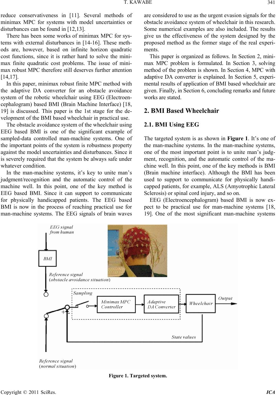

T. KAWABE341
reduce conservativeness in [11]. Several methods of
minimax MPC for systems with model uncertainties or
disturbances can be found in [12,13].
There has been some works of minimax MPC for sys-
tems with external disturbances in [14-16]. These meth-
ods are, however, based on infinite horizon quadratic
cost functions, since it is rather hard to solve the mini-
max finite quadratic cost problems. The issue of mini-
max robust MPC therefore still deserves further attention
[14,17].
In this paper, minimax robust finite MPC method with
the adaptive DA converter for an obstacle avoidance
system of the robotic wheelchair using EEG (Electroen-
cephalogram) based BMI (Brain Machine Interface) [18,
19] is discussed. This paper is the 1st stage for the de-
velopment of the BMI based wheelchair in practical use.
The obstacle avoidance system of the wheelchair using
EEG based BMI is one of the significant example of
sampled-data controlled man-machine systems. One of
the important points of the system is robustness property
against the model uncertainties and disturbances. Since it
is severely required that the system be always safe under
whatever condition.
In the man-machine systems, it’s key to unite man’s
judgment/recognition and the automatic control of the
machine well. In this point, one of the key method is
EEG based BMI. Since it can support to communicate
for physically handicapped patients. The EEG based
BMI is now in the process of reaching practical use for
man-machine systems. The EEG signals of brain waves
are considered to use as the urgent evasion signals for the
obstacle avoidance system of wheelchair in this research.
Some numerical examples are also included. The results
give us the effectiveness of the system designed by the
proposed method as the former stage of the real experi-
ments.
This paper is organized as follows. In Section 2, mini-
max MPC problem is formulated. In Section 3, solving
method of the problem is shown. In Section 4, MPC with
adaptive DA converter is explained. In Section 5, experi-
mental results of application of BMI based wheelchair are
given. Finally, in Section 6, concluding remarks and future
works are stated.
2. BMI Based Wheelchair
2.1. BMI Using EEG
The targeted system is as shown in Figure 1. It’s one of
the man-machine systems. In the man-machine systems,
one of the most important point is to unite man’s judg-
ment, recognition, and the automatic control of the ma-
chine well. In this point, one of the key methods is BMI
(Brain machine interface). Although the BMI has been
used to support to communicate for physically handi-
capped patients, for example, ALS (Amyotrophic Lateral
Sclerosis) or spinal cord injury, and so on.
EEG (Electroencephalogram) based BMI is now ex-
pect to be practical use for man-machine systems [18,
19]. One of the most significant man-machine systems
Figure 1. Targeted system.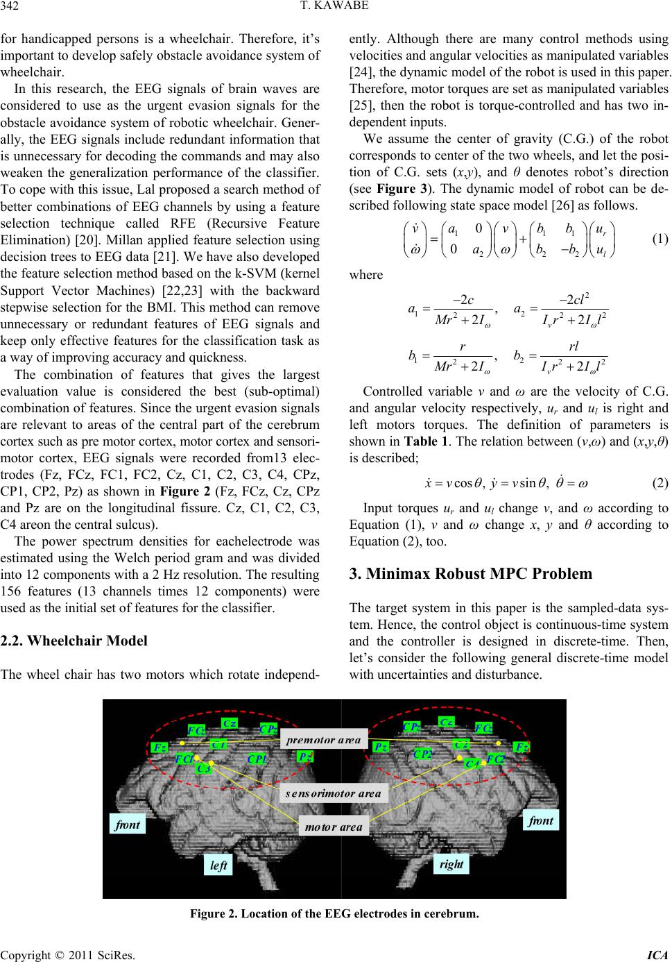

T. KAWABE 342
for handicapped persons is a wheelchair. Therefore, it’s
important to develop safely obstacle avoidance system of
wheelchair.
In this research, the EEG signals of brain waves are
considered to use as the urgent evasion signals for the
obstacle avoidance system of robotic wheelchair. Gener-
ally, the EEG signals include redundant information that
is unnecessary for decoding the commands and may also
weaken the generalization performance of the classifier.
To cope with this issue, Lal proposed a search method of
better combinations of EEG channels by using a feature
selection technique called RFE (Recursive Feature
Elimination) [20]. Millan applied feature selection using
decision trees to EEG data [21]. We have also developed
the feature selection method based on the k-SVM (kernel
Support Vector Machines) [22,23] with the backward
stepwise selection for the BMI. This method can remove
unnecessary or redundant features of EEG signals and
keep only effective features for the classification task as
a way of improving accuracy and quickness.
The combination of features that gives the largest
evaluation value is considered the best (sub-optimal)
combination of features. Since the urgent evasion signals
are relevant to areas of the central part of the cerebrum
cortex such as pre motor cortex, motor cortex and sensori-
motor cortex, EEG signals were recorded from13 elec-
trodes (Fz, FCz, FC1, FC2, Cz, C1, C2, C3, C4, CPz,
CP1, CP2, Pz) as shown in Figure 2 (Fz, FCz, Cz, CPz
and Pz are on the longitudinal fissure. Cz, C1, C2, C3,
C4 areon the central sulcus).
The power spectrum densities for eachelectrode was
estimated using the Welch period gram and was divided
into 12 components with a 2 Hz resolution. The resulting
156 features (13 channels times 12 components) were
used as the initial set of features for the classifier.
2.2. Wheelchair Model
The wheel chair has two motors which rotate independ-
ently. Although there are many control methods using
velocities and angular velocities as manipulated variables
[24], the dynamic model of the robot is used in this paper.
Therefore, motor torques are set as manipulated variables
[25], then the robot is torque-controlled and has two in-
dependent inputs.
We assume the center of gravity (C.G.) of the robot
corresponds to center of the two wheels, and let the posi-
tion of C.G. sets (x,y), and θ denotes robot’s direction
(see Figure 3). The dynamic model of robot can be de-
scribed following state space model [26] as follows.
111
222
0
0
r
l
u
abb vv
u
abb 
    

    
 
  

 (1)
where
2
12
22
22
,
22
v
cc
aa
2
l
M
rI IrIl




12
22
,
22
v
rr
bb
2
l
M
rI IrIl



Controlled variable v and ω are the velocity of C.G.
and angular velocity respectively, ur and ul is right and
left motors torques. The definition of parameters is
shown in Table 1. The relation between (v,ω) and (x,y,θ)
is described;
cos, sin, xv yv

 



 
(2)
Input torques ur and ul change v, and ω according to
Equation (1), v and ω change x, y and θ according to
Equation (2), too.
3. Minimax Robust MPC Problem
The target system in this paper is the sampled-data sys-
tem. Hence, the control object is continuous-time system
and the controller is designed in discrete-time. Then,
let’s consider the following general discrete-time model
with uncertainties and disturbance.
Figure 2. Location of the EEG electrodes in cerebrum.

T. KAWABE 343
Figure 3. Model of robotic wheelchair.
Table 1. Definition of parameters.
I

Inertia moment [Nms2/rad]
M Weight [Kg]
v
I
Inertia moment of rotation center [Nms2/rad]
l Distance between wheel and rotation center [m]
c Viscosity coefficient of friction [Nms2/rad]
r Wheel radius [m]

1AB

x
kALRxkBLRu k (3)
 
()
y
kCxk k   (4)
where x(k), u(k), y(k) and η(k) denote the state, input,
measure doutput and disturbance vector respectively, and
where is a diagonal structured uncertain parameters
matrix satisfied

ΔΔ
T
I
. L, RA and RB are constant ma-
trices. All these vectors and matrices have appropriate
dimensions. Then, we can transform this system as
 
1
x
kAxkBu k (5)
 
AB
zkRxkRuk (6)
 
y
kCxk k   (7)
where w(k)(:=Δz(k)). We assumed that the system is con-
strained with following conditions;



1
T
w
wk jPwk j



1
TkjP kj

 

 
1
T
u
ukjPukj




0, ,1jN


where P
w, P η, P u are positive symmetric matrices for
weights of constraints. For this system, the quadratic
performance measure with finite horizon with positive
weighting constant matrices Q and R as :
 


122
0
1
N
QR
j
Jkyk jkuk jk



 (8)
is used. x(k + j|k), y(k + j|k) and u(k + j|k) are the pre-
dicted state of the plant, the predicted output of the plant
and the future control input at time k + j respectively.
Then, the design problem is formulated as the following
minimax optimization problem.
 

||, |
min m ax
uk jkwkjkkjk
J
k
  (9)
subject to

 
1
T
w
wk jPwk j



 
1
TkjP kj





 
1
T
u
ukjPukj




0, ,1jN


Since the saddle point may not exist in general, it is
difficult to solve this problem. Hence, the objective is to
eliminate the maximization procedure and transform this
problem to simple minimization problem which can be
solved easily.
4. Transformation of the Problem
At each step k the following state feedback is employed;


kj
ukjkF xkjk

 

(10)
where Fk+j is a feedback gain matrix. Then, introducing
the following vectors

1T XxkkxkNk


 


:

1T YykkykNk


 


:
 
1T UukkukNk





:
 
1T WwkkwkNk





:
 
Λ1T kkk Nk 





:
and using state space equation, Equations (5)-(7), recur-
sively, we can derive


T. KAWABE 344

X
Ax kBULW

(11)

ΛYCAxk CLW
 (12)
where
21
T
N
AAA A




:
23
00
0
NN
B
AB B
B
A
BA BB












:


23
00
0
NN
L
AL L
L
A
LA LL












:





Hence, we can transform the minimax problem (9) to
min
U

(13)
subject to
,Λ
max Π
W





1
T
w
wk jPwk j



1
TkjP kj

 



1
T
u
ukjPukj

0, ,1jN
where γ > 0 (scalar parameter) and where;

22
ˆ
ˆ
ΠΛ
R
Q
A
xkBULWU

:,
00
ˆˆ
,
00
QR
QR
QR






::













To eliminate the maximaization procedure, we have to
remove W and terms in the first constraint. For this,
in the first place, following basis for all variables and
transformation matrices are defined.


Λ1T
TT
xkW 

 (14)

0
uu
U HHFAFLF 




: (15)

0
yy
YH HCACLI 




: (16)



Λ00 0

H
HI

 : (17)

 
111
10
T
HHH  : 01 (18)
where
1
1
00
0
0
0 0
k
k
kN
F
F
F
F




















 

:
By using these, we can express the first constraint
condition of problem (13);



ˆ
,Λ
22
max T
yu
Q
WHH HH
ˆ11
R
 


 (19)
Please take notice that both the left side and t
side of this inequality are expressed by the quadratic
fo
he right
rms and they have positive scalar values. Hence, if the
inequality is hold by maximum values of W and

in
left side, this inequality must be hold by any other values
of them. This fact means that we can eliminate the
maximization procedure in the first constraint. We can
only check the following condition instead of the first
constraint of problem (13).

1
2
ˆ
ˆ
2T
yu
R
Q
HH HH
1



 (20)
In the second place, $H_{w}(j)$ is defined
trix pick out the suitable block from W and satisfy the
re
. This ma-
lation of



0,,1.
j
w
wk jHjN 

Then, we
can derive







11
TT
jj
www
PHHHH

 (21)
For the constraints of η and u, we can deri
lowing relations in the same way.
ve the fol-







TT
jj
HPH H


11
H

 (22)







11
TT
jj
uuu
HPH HH


 (23)
Then, by using (14)-(19), all constraints i
problem (13) can be transformed into:
n minimax












11
11
11
0
0
0
0
ζ0
u
T
jj
TT
www
T
jj
TT
T
jj
TT
uuu
HH H PH
HH HPH
HH HPH





11 ˆˆ
TT TT
yy u
HH HQHHRH 


(24)
We can transform the original minimax problem (9) to
the following one by using S-procedure [27].













min
F

(25)

T. KAWABE345
subject to
11
1
0
ˆˆ
,
TT T
yy uu
Nww uu
jjjj jj
j
HH HQHHRH
SSS











 
where
ww






uu

and where



11
T
jj
wT
jw
SHHHPH







11
T
jj
T
j
SHHHPH









11
T
jj
uT
ju
SHHHPH




wu
,,
j
jj



noted that t
are positive semi-deite scalars.
It must be his transformation satisfies only a
9) into the following
pr
fin
sufficient condition of S-procedure, since S-procedure is
not the so-called “lossless” in this case. We cannot there-
fore avoid that the design results are slightly conserva-
tive. Nevertheless, we can expect the reduction of con-
servativeness in design result by this technique in con-
trast with the results by preexisting methods. Because the
conservativeness caused by S-procedure is too small to
put a matter for practical purposes.
Finally, using “Schur-complement” [28], we can trans-
formed the minimization problem (
oblem which can be solved easily by using some opti-
mization tool.
min
F

(26)
subject to
where

11
1
1
Σ
ˆ00
ˆ
0
,,0 0,,1
TTT
yu
y
u
wu
jjj
HHH H
HQ
HR
jN













 
,
1
0
Σ
Nwwuu
j
jjjjj
j
SSS








:,
ith Adaptive DA Converter
pling points is
eed for getting the current control input by the interpo-
ly fast-moving dynamics, such as robots or vehi-
cl
5. MPC w
5.1. Interpolation of Control Inputs
Although the information about future sam
n
lating operations of the sampled-data control systems,
it’s impossible to obtain them. Therefore, we have been
forced to tolerate the long time-delay during the DA
conversion to wait for getting the indispensable informa-
tion.
However, in the case of controlling the systems with
relative
es, the method with long time-delay is unable to be
applied. Furthermore, it takes much computation time to
calculate the interpolation by using the high-order sam-
pling functions to DA conversion in sampled-data con-
trol system.Therefore a new idea to use the predictive
control inputs obtained by MPC for interpolation is pro-
posed.
In MPC algorithm, the optimal control inputs




 
ˆ
,, 1ukk N
ˆ
ukk

 are calculated in each step,
and only the first control input

ˆ
ukk is used a
e consider to use the other
optimal control inputs
s a real
control input.Therefore, w




1,
hich are neede
ˆ
ukk as virtual future
sampling points.Actually, it is only necessary to use the
optimal control inputs wd for interpolation
according to the sampling function.
Figure 4 shows this way using the 2nd order spline
function for interpolations. Only

ˆ
u1kk is used as a
vi
oints and real
sa
rtual future sampling point in this case. By using the
predictive control inputs for interpolation, it becomes
possible to reduce the time-delay in the DA conversion,
and the total time-delay to be needed is just only compu-
tation time of optimization in current step.
Of course, it needs to take account that there is a dif-
ference between virtual future sampling p
mpling points like



ˆˆ
11ukkuk

 in future step.
However, we consider that this point is not a critical
problem because the ated waveform
due to prediction error is not so big compared to the scale
of prediction error. Although the differentiability of each
sampling function is lost at sampling points, this also
does not become a critical problem compared to the
influence on interpol
Figure 4. Interpolation based on a 2nd order spline sam-
pling function using predictive future control inputs.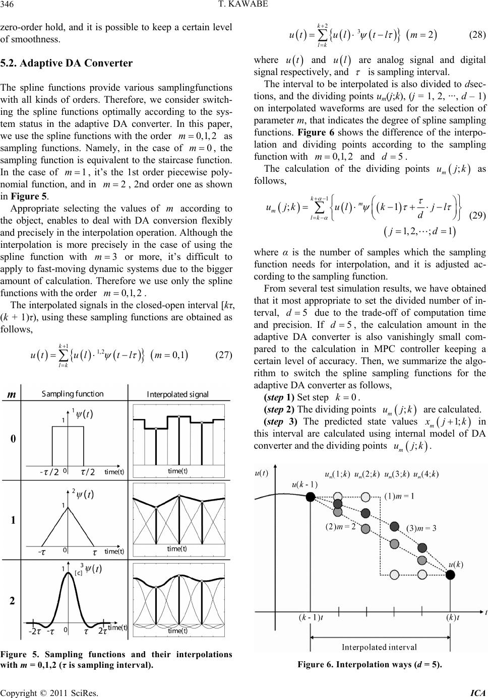

T. KAWABE 346
A Converter
us samplingfunctions
zero-order hold, and it is possible to keep a certain level
of smoothness.
5.2. Adaptive D
The spline functions provide vario
with all kinds of orders. Therefore, we consider switch-
ing the spline functions optimally according to the sys-
tem status in the adaptive DA converter. In this paper,
we use the spline functions with the order 0,1,2m as
sampling functions. Namely, in the case of 0m

, the
sampling function is equivalent to the staircase fuon.
In the case of 1m, it’s the 1st order piecewise poly-
nomial function, and in 2m, 2nd order one as shown
in Figure 5.
Appropriate selecting alues of m according to
the object, en
ncti
the v
(27)
ables to deal with DA conversion flexibly
and precisely in the interpolation operation. Although the
interpolation is more precisely in the case of using the
spline function with 3m or more, it’s difficult to
apply to fast-moving dynamic systems due to the bigger
amount of calculation. Therefore we use only the spline
functions with the order 0,1, 2m.
The interpolated signals in the closed-open interval [kτ,
(k + 1)τ), using these sampling functions are obtained as
follows,

ut





11,2 0,1 k
lk
ult lm 




Figure 5. Sampling functions and their interpolations
with m = 0,1,2 (τ is sampling interval).
2
   


23 k
lk
utultlm 



 
 (28)
where


ut and


ul
and
are analog signal and digital
signal respectively,

is sampling interval.
e int
oi , d – 1)
on
The interval to berpolated is also divided to dsec-
tions, and the dividing pnts um(j;k), (j = 1, 2, ···
interpolated waveforms are used for the selection of
parameter m, that indicates the degree of spline sampling
functions. Figure 6 shows the difference of the interpo-
lation and dividing points according to the sampling
function with 0,1,2m

and 5d.
The calculation of the dividing points


;
m
ujk as
follows,
 

1
;
k
m
ujk


1
1,2,;1
m
lk
ul kjl
d
jd

















(29)
where α is the number of samples which the sampling
function needs for interpolation, and it is adjusted ac-
ivided number of in-
te
cording to the sampling function.
From several test simulation results, we have obtained
that it most appropriate to set the d
rval, 5d

due to the trade-off of computation time
and precision. If 5d

, the calculation amount in the
adaptive converter is also vanishingly small com-
pared to the calculation in MPC controller keeping a
certain level of accuracy. Then, we summarize the algo-
rithm to switch the spline sampling functions for the
adaptive DA converter as follows,
(step 1) Set step 0k
DA

.
(step 2) The dividing points

m
uj;k
values
are calculated.
dicted state (step 3) The pre

1;
m
x
jk

.
in
this interval are calculated using intern
co
al model of DA
nverter and the dividing points

;
m
ujk
Figure 6. Interpolation ways (d = 5).

T. KAWABE 347
(step 4) If the interpolation waves exceeds the c
strained conditions of control input due to the oversho
or undershoot, this is excluded.
(step 5) The evaluation values of evaluation function
on-
ot
 If the signal 1 or −1 is detected, the wheelchair does
the evasion run in a specified direction according to
half oval orbit. The radius of half oval changes ac-
cording to value of the signal.
Now we assume the following perturbations of l and c
in the wheelchair model.
m

J
k
(step
od Equation (8) are calculated in each .
6) The parameter whose evaluatio value is
the smallest is selected as an interpolation way in this
interval, and then nd go back to (step1).
6. Numerical Experiments
The experimental conditions are summarized as follows.
 The robotic wheelchair goes straight according to the
reference path usually.
 The signal from the BMI was read at constant inter-
vals (100 ms).
 The sihe signal
h and −1 has 0 - 1.
m
nm
1 akk


0.08 0.12ll l,


0.03 0.07cc c
The weights of the cost function in Equation (8) are
125 00.550
,
0 1500.15
QR





 

 
Figures 7-10 show simulation results with various
conditions. The parameter r = 0.2 [m]. The size of obsta-
cle is different between Figures 7 and 8, but initial posi-
tion of obstacle is same. Figs. 9and 10 show the two ob-
stacle case. In Figures 7-9, red line indicates the nearest
trajectory of the center of gravity (C.G.) of robotic wheel
gnal classified the three types: 0 (t
none), 1 or −1 (left or right evasion). 1 and −1 are the
emergent evasion signals against the obstacle appear-
ed suddenly. Eacvalue of signals 1
Figure 7. The C.G. trajectories (a).
Figure 8. The C.G. trajectories (b).

T. KAWABE 348
Figure 9. The C.G. trajectories (c).
Figure 10. The C.G. trajectories (d).
chair to the obstacle against the perturbation of model
uncertainties. Blue line indicates the furthest one. All
results show that thewheelchair can avoid the obstacle
safely even if parameter uncertainties are existing. For
the comparison, in the case of using the standard MPC
instead of the proposed minimax MPC, the wheelchair
had collided with the obstacle whenever the parameters
(l and c) were perturbed even if no collision occurred
with the nominal values of l and c. Since the standard
MPC is a nominal control method and it cannot guaran-
tee the robustness property against the parameter pertur-
bations.Hence, we can easily see that the proposed
method have good robust performance against the model
uncertainties and we can recognize the effectiveness of
the proposed method.
. Conclusions
As the first stage of the development of the BMI based
wheelchair system, new minimax robust MPC method
with the adaptive DA converter applied to the obstacle
avoidance system in the BMI based wheelchair has been
proposed. Simulation results have been illustrated to in-
dicate the good robust performance as the development
of the former stage of real experimental system. From
these results, the proving test by the real experiments of
the BMI based wheelchair by the real experiments will
be done in next stage.
In addition to, the proposed minimax MPC method is
easily extended the systems with other constraints which
are specified by ellipsoidal bounds, for example, state
estimation errors and so on as follows. In the case that
x(k) is not full measured and we need to estimate x(k),
where the bound of estimation error
7





ˆ ekxk kx
is guaranteed an ellipsoidal set as:


ee
T
e
kP k 1
e
where, P is a positive symmetric matrix for weight. This

T. KAWABE349
specification of estimation error is standard one. Now we
introduce He as:

ˆ
10 0
e
H
xk 

:
then the relation of e(k) = He

is hold. And the condi-
tion below is also hold.



11 0
T
jj
TT
eee
HH HPH 




Since this condition has same form as other constraints
in Equation (24), we can include this condition into the
condition of problem (25) by using a new variable e
j

.
8. References
[1] C. E. Garcia, D. M. Prett and M. Morari, “Model Predic-
tive Control: Theory and Practice—A Survey,” Automatica,
Vol. 25, No. 3, 1989, pp. 335-348.
doi:10.1016/0005-1098(89)90002-2
[2] J. Ackermann, “Sampled-Data Control Systems: Analysis
and Synthesis, Robust System Design,” Springer-Verlag,
Berlin, 1985.
[3] P. T. Kabamba, “Control of Linear Systems Using Gener-
alized Sampled-Data Hold Functions,” IEEE Transactions
on Automatic Control, Vol. 32, No. 9, 1987, pp. 772-783.
doi:10.1109/TAC.1987.1104711
[4] B. D. O. Anderson, “Controller Design: Moving from The-
ory to Practice,” IEEE Control Systems Magazine, Vol. 13,
No. 4, 1983, pp. 16-25. doi:10.1109/37.229554
[5] Y. Yamamoto, “A Function Space Approach to Sampled-
Data Control Systems and Tracking Problems,” IEEE Tran-
sactions on Automatic Control, Vol. 39, No. 4, 1994, pp.
703-713. doi:10.1109/9.286247
[6] D. R. Ramirez and E. F. Camacho, “Piecewise Affinity of
Min-Max MPC with Bounded Additiveuncertainties and
a Quadratic Criterion,” Automatica ol. 42, No. 2, 2006, , V
pp. 295-302. doi:10.1016/j.automatica.2005.09.009
[7] A. Grancharova and T. A. Johansen, “Computation, Ap-
proximation and Stability of Explicit Feedback Min-Max-
Nonlinear Model Predictive Control,” Automatica, Vol.
45, No. 5, 2009, pp. 1134-1143.
doi:10.1016/j.automatica.2008.12.023
[8] P. J. Campo and M. Mora, “Robust Model Predictive
Control,” Proceeding
ri
s of 1987 American Control Con-
ference, Minneapolis, 10-12 June 1987, pp. 1021-1026.
[9] Z. Q. Zheng and M. Morari, “Robust Stability of Con-
strained Model Predictive Control,” Proceedings of 1987
r -
” Automatica, Vol. 32, No. 10, 1996, pp.
i:10.1016/0005-1098(96)00063-5
American Control Conference, San Francisco, 2-4 June
1993, pp. 379-383.
[10] M. V. Kothare, V. Balakrishnan and M. Morari, “Robust
Constrained Model Predictive Control using LineaMa
trixInequalities,
1361-1379. do
September 2001, pp.
nses,” System & Control Letters, Vol. 18,
[11] F. A. Cuzzola, J. C. Geromel and M. Morari, “An Im-
proved Discrete-Time Robust Approach for Constrained
Model Predictive Control,” Proceedings of 2001 Euro-
pean Control Conference, Porto, 4-7
2759-2764.
[12] J. C. Allwright and G. C. Papavasiliou, “On Linear Pro-
gramming and Robust Model-Predictive Control Using
Impulse-Respo
No. 2, 1992, pp. 159-164.
doi:10.1016/0167-6911(92)90020-S
[13] J. H. Lee and Z. Yu, “Worst-Case Formulation of Model
Predictive Control for Systems with Bounded Parame-
ters,” Automatica, Vol. 33, No. 5, 1997, pp. 768-781.
doi:10.1016/S0005-1098(96)00255-5
[14] A. Bemporad and M. Morari, “Robust Model Predictive
26.
Control: A Survey,” In: A. Garulli, A. Tesi and A. Vicino,
Eds., Robustness in Identification and Control, Lecture
Notes in Control and Information Sciences, Vol. 245,
Springer-Verlag, 1999, pp. 207-2
[15] A. Bemporad and A. Garulli, “Output-Feedback Predic-
tive Control of Constrained Linear Systems via Set-Mem-
bership State Estimation,” International Journal of Con-
trol, Vol. 73, No. 8, 2000, pp. 655-665.
doi:10.1080/002071700403420
[16] P. O. M. Scokaert and D. Q. Mayne, “Min-Max Feedback
Model Predictive Control for Constrained Linear Sys-
tems,” IEEE Transactions on Auto
No. 8, 1998, pp. 1136-1142.
matic Control, Vol. 43,
9/9.704989doi:10.110
.
[17] D. Q. Mayne, J. B. Rawlings, C. V. Rao and M. Scokaert,
“Constrained Model Predictive Control: Stability and Op-
timality,” Automatica, Vol. 36, No. 6, 2000, pp. 789-814
doi:10.1016/S0005-1098(99)00214-9
[18] S. Waldert, T. Pistohl, C. Braun, T. Ball, A. Aertsen and C.
Mehring, “A Review on Directional Information in Neural
Signals for Brain-Machine Interfaces,” Journal of Physi-
ology Paris, Vol. 103, No. 3-5, 2009, pp. 244-254.
doi:10.1016/j.jphysparis.2009.08.007
[19] R. Heliot and J. M. Carmena, “Brain-Machine Inter-
faces,” Encyclopedia of Behavioral Neuroscience, 2010,
pport Vector Channel Selection in BCI,”
pp. 221-225.
http://www.sciencedirect.com/science/article/pii/B97800
80453965002098
[20] T. N. Lal, M. Schroder, T. Hinterberger, J. Weston and M.
Bogdan, “Su
IEEE Transactions on Biomedical Engineering, Vol. 51,
No. 6, 2004, pp. 1003-1010.
doi:10.1109/TBME.2004.827827
[21] J. del R. Millan, M. Franze, J. Mouri
Babiloni, “Relevant EEG Features f
no, F. Cincotti and F.
or the Classification
of Spontaneous Motor-Related Tasks,” Biological Cyber-
netics, Vol. 86, No. 2, 2002, pp. 89-95.
doi:10.1007/s004220100282
[22] V. N. Vapnik, “Statistical Learning Theory,” John Wiley
010
& Sons, New York, 1998.
[23] C. T. Suand and C. H. Yang, “Feature Selection for the
SVM: An Application to Hypertension Diagnosis,” Ex-
pert Systems with Applications, Vol. 34, No. 1, 2008, pp.
754-763. doi:10.1016/j.eswa.2006.10.
[24] M. Sampei and M. Ishikawa, “State Estimation and Out-
put Feedback Control of Nonholonomic Mobile Systems

T. KAWABE 350
tion Engineers
3.
D-R
using Time-Scale Transformation,” Transactions of the
Institute of Systems, Control and Informa
Vol. 13, No. 3, 2000, pp. 124-13
,
[25] R. Fierro and F. L. Lewis, “Control of a Nonholonomic Mo-
bile Robot: Backstepping Kinematics into Dynamics,” Jour-
nal of Robotic Systems, Vol. 14, No. 3, 1997, pp. 149-163.
doi:10.1002/(SICI)1097-4563(199703)14:3<149::AI
OB1>3.0.CO;2-R
[26] J. Tang, K. Watanabe, M. Nakamura and N. Koga, “Fuz-
zy Gaussian Neural Network Controller and Its Applica-
tion to the Control of a Mobile Robot,” Transactions of
Japan Society of Mechanical Engineers, Series C, Vol. 59,
No. 564, 1993, pp. 2290-2297.
[27] S. Boyd and C. H. Barratt, “Linear Controller Design: Li-
mits of Performance,” Prentice-Hall, Upper Saddle River,
1991.
[28] K. Zhou, J. C. Doyle and K. Glover, “Robust and Opti-
mal Control,” Prentice-Hall, Upper Saddle River, 1996.