Intelligent Control and Automation, 2011, 2, 293-298
doi:10.4236/ica.2011.24034 Published Online November 2011 (http://www.SciRP.org/journal/ica)
Using the Prony Analysis for Assessing Servo Drive Control
Reimund Neugebauer, Ruben Schönherr*, Holger Schlegel
Chemnitz University of Technology, Faculty of Mechanical Engineering, Institute for Machine Tools
and Production Processes, Chemnitz, Germany
Received June 10, 2011; revised July 1, 2011; accepted August 8, 2011
Abstract
The Prony Analysis is already used in different fields of science and industries. The described new approach
intends assessing the performance of Servo Drive Control. The basic approach is, that two important dy-
namic parameters of closed loop behavior, damping and frequency, are estimated by the Prony method.
Hence analyzing a control loop in this way leads to a statement concerning the quality of control and allows
comparing different parameter sets. The paper presents results achieved by using this method on a test rig.
Keywords: Servo Drive, Control, Assessment, Monitoring, Prony Method
1. Introduction
Several mathematical approaches proofed to be practical
for monitoring functions and assessment purposes in
refineries and chemical plants. Therefore, automatic con-
troller assessment is a known feature of state-of-the-art
process controlling systems. The most common term in
literature for these methods is “Control Loop Perform-
ance Monitoring” (CLPM).
Observing the controller behaviour of servo drives in a
similar way ought to be advantageous for machines in
production industries. Due to a raising number of direct
drives and lightweight components, controller settings
have a growing influence on the overall system behav-
iour. Thus, detecting inadequate control characteristics
becomes also more important for process reliability.
Furthermore, monitoring methods could contribute to the
reduction of energy consumption in the drive by auto-
matically recognizing aggressively tuned controllers.
The idea of implementing the known methods in drive
controllers is the most obvious way in order to benefit
from the research in the field of process control moni-
toring. However, several differences between the two
fields of controlling impede this direct approach. The
main drawback results from the different objectives of
controlling:
In process industries, control is focused on keeping the
controlled variable close to a constant setpoint. Thus
disturbance rejection is of major importance. In com-
parison to this, drive systems are supposed to follow a
dynamically changing setpoint. So, emphasis is placed
on tracking capabilities. The following Ta ble 1 points
out to further differences between process and servo
drive control.
Because of these disparate properties, the known
methods of CLPM can not easily be implemented into
drive systems. Especially the traditional attributes for
assessing controller performance like output variance [2]
are not suitable for drive systems. This leads to a need
for new methods of controller assessment in the field of
servo drives.
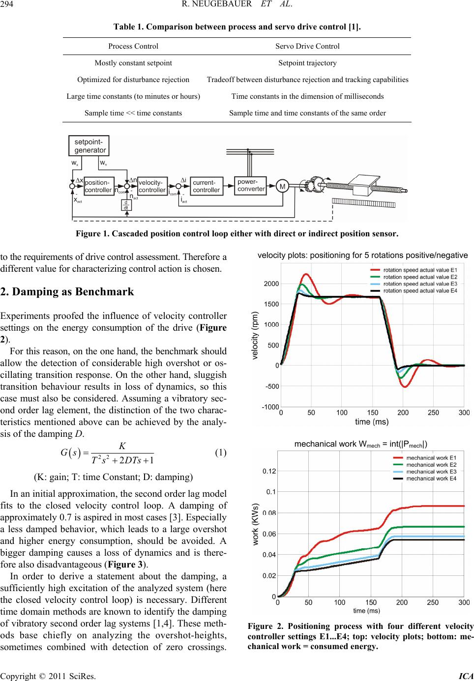
Servo Drive Control
Appart from some special applications, the cascaded
loop structure shown in Figure 1 is the basis of most
controlled (electrical) drive systems [3].
The paper focuses on the velocity feedback control of
electrical servo drives because of different reasons. Two
should be mentioned here:
Firstly, monitoring of the current control loops behav-
iour is not expected to be very useful, because it depends
on the well known or measurable parameters inductance
and resistance. So automatic tuning is state of the art and
leads to feasible results. Furthermore parameters are
nearly constant over time, so deterioration of behavior is
not expected.
Secondly, the velocity controllers’ behavior limits the
achievable dynamics of the position controller. So the
velocity control loop is of major importance regarding
the drive dynamics.
As mentioned above, the quantity “variance of control-
led variable” commonly used as benchmark, does not suit

R. NEUGEBAUER ET AL. 294
Table 1. Comparison between process and servo drive control [1].
Process Control Servo Drive Control
Mostly constant setpoint Setpoint trajectory
Optimized for disturbance rejection Tradeoff between disturbance rejection and tracking capabilities
Large time constants (to minutes or hours)Time constants in the dimension of milliseconds
Sample time << time constants Sample time and time constants of the same order
Figure 1. Cascaded position control loop either with direct or indirect position sensor.
to the requirements of drive control assessment. Therefore a
different value for characterizing control action is chosen.
2. Damping as Benchmark
Experiments proofed the influence of velocity controller
settings on the energy consumption of the drive (Figure
2).
For this reason, on the one hand, the benchmark should
allow the detection of considerable high overshot or os-
cillating transition response. On the other hand, sluggish
transition behaviour results in loss of dynamics, so this
case must also be considered. Assuming a vibratory sec-
ond order lag element, the distinction of the two charac-
teristics mentioned above can be achieved by the analy-
sis of the damping D.

22 21
K
Gs Ts DTs  (1)
(K: gain; T: time Constant; D: damping)
In an initial approximation, the second order lag model
fits to the closed velocity control loop. A damping of
approximately 0.7 is aspired in most cases [3]. Especially
a less damped behavior, which leads to a large overshot
and higher energy consumption, should be avoided. A
bigger damping causes a loss of dynamics and is there-
fore also disadvantageous (Figure 3 ).
In order to derive a statement about the damping, a
sufficiently high excitation of the analyzed system (here
the closed velocity control loop) is necessary. Different
time domain methods are known to identify the damping
of vibratory second order lag systems [1,4]. These meth-
ods base chiefly on analyzing the overshot-heights,
sometimes combined with detection of zero crossings.
velocity plots: positioning for 5 rotations positive / negative
mechanical work Wmech = int(|Pmech|)
Figure 2. Positioning process with four different velocity
controller settings E1...E4; top: velocity plots; bottom: me-
chanical work = cons umed energy.

R. NEUGEBAUER ET AL.295
Figure 3. Aspired damping of the closed velocity control
loop.
However this is disadvantageous for drive controllers:
Because of sampling and measurement noise, evaluat-
ing a single value (such as the maximum over-/undershot)
tends to contain errors. In addition the overshot is quite
small, especially for D > 0.6.
The measuring time (for example to analyze zero
crossings) is limited to the sampling rate of the controller
and therefore not accurate enough.
The approach described here uses the Prony Analysis
to evaluate the damping of the closed velocity controller
to avoid these disadvantages. This method proofed to be
more efficient concerning this task than the ones men-
tioned above. In the following section, the approach is
briefly described before some of the results will be pre-
sented.
3. Prony Method
Similarly to the Fourier transform, the Prony method is
used to analyze a measured signal and to gain spectral
information. Unlike the Fourier transform, the signal is
described by damped sinusoids. This property makes
Prony analysis suitable for the task of evaluating the
damping factor.
3.1. Approach
The analysis is based on the following equations, de-
scribing the evenly sampled signal as a sum of p damped
sinusoids in the complex Euler representation, where N
is the number of samples:
1
; 1,2;3;;
pnt
mm
m
x
bz nN


 
 (2)
ˆe; e
mm
j
mm m
bA zm
j

 
  (3)
Âm … mth amplitude,

m … mth phase,

m … mth damping factor,
ωm … mth circular frequency,
t … sample time
For N > 2p, the extended Prony Method is used. This
includes solving the overdetermined set of equations
utilizing a least squares approach [5]. The derivation of
the whole method would go beyond the scope of the pa-
per, so just a short outline of the algorithm is given. The
procedure can be divided in three major steps:
1) Solve linear prediction model to gain characteristic
polynomial (least squares method);
2) Calculate complex roots of characteristic polyno-
mial ( frequency and damping factor arise);
3) Solve (overdetermined) set of linear equations (
amplitude and phase arise).
The result is an approximation containing p/2 sinu-
soids (negative frequencies are omitted) of the analyzed
signal. The computational effort is bigger compared to
other calculation methods for the damping, but there are
several advantages which will be described in the next
section.
3.2. Assessing the Velocity Controller
The basic idea is the calculation of the damping of a vi-
bratory second order lag system (1). For this purpose

R. NEUGEBAUER ET AL. 296
Prony Analysis is used on a system response in the time
domain. To simplify the derivation here, an impulse re-
sponse h(t) and a step response a(t) of a vibratory second
order lag system are utilized [4]:
 
 
22
1
2
ˆ
21
1esin
D
Te
h
K
Hs GssTs DTs
L
htKD Tt





 
  ;

(4)
 

 
22
1
2
ˆ
21
esin
1
D
Te
a
K
As GssTs DTss
L
K
at Kt
D




 

 

 
(5)
21
1
eDT
  

arccos D  
Using Euler’s relation in (2) and (3) with a single si-
nusoid in continuous time yields:


  
ˆee
ˆecos sin
j
jt
t
xt A
Atjt










  
(6)
The complex part can be omitted, since a real signal is
analyzed.
 
ˆecos
αt
xt At



 (7)
By writing (4) and (5) as deviation from the steady
state
 
ˆesin
D
Te
ht ht



 
 (8)
 
ˆesin
D
Te
at at

;



 
 (9)
and comparing (7) with (8) and (9), the following rela-
tions between the parameters can be derived:
2
11
eD
T
  (10)
D
T
  (11)
ˆimpulse
ˆstep
ˆ
h
Aa






 (12)
πimpulse
2
πstep
2











(13)
Obviously, the relations between ω,  and T, D are
independent from the excitation. This is evident, because
these terms describe the free oscillation of the system.
Parameters of a vibratory second order lag system are
calculated based on the results of a Prony Analysis by
Equations (10) and (11). Equations (12) and (13) reveal
that amplitude and phase depend on the actual excitation.
Conversely, a different excitation only effects  and Φ.
The Prony Analysis yields information of frequency,
damping factor, amplitude and phase. Assuming a con-
trol without steady state error, the closed loop gain is
always equal one. Therefore, the closed velocity loop
modeled as vibratory second order lag system is com-
pletely described by the two parameters T and D. So,
theoretically the third step for calculating the amplitude
and the phase could be omitted. However, the amplitude
is a suitable value, to identify irrelevant sinusoids in the
system response, if the chosen model order is greater
than one. For this purpose, a rather rough estimate of
amplitude is sufficient. Hence, a significant reduction of
equations in the third step of the algorithm is tolerable.
Thus, the Gaussian Algorithm can be utilized and com-
putational effort can considerably be reduced.
Literature points out some drawbacks of the Prony
Analysis [6], especially poor behavior if there is noise
present in the observed signal and the signal to noise
ratio is low.
Due to confining the analysis to a time period after an
excitation of the closed control loop, the signal noise is
uncritical in case of the proposed drive controller as-
sessment. On the contrary, the calculation of frequency is
less sensitive to measurement errors compared to other
methods in the time domain. This is because, in contrast
to these other approaches, the calculation of frequency is
not based on the measurement of concrete zero crossings.
As described above it is based on a least squares fit (step
one of the algorithm) and therefore averaged over the
whole measurement duration. For the same reason, the
frequency resolution additionally is not limited by the
length of the analyzed data but only by the sample time.
This is also one advantage in comparison to the Fourier
Analysis. Moreover, the Prony Analysis is based on a
parametric approach, which facilitates the automatic in-
terpretation of the results significantly.
4. Results
The Prony Analysis was applied for velocity controllers
of different test rigs. Because of the provided excitation,
the characteristics of different controller settings were
correctly identified.
Best results were achieved with a measurement dura-
tion of 100 to 300 samples and a quite small number of
sinusoids (2 to 4) with positive frequencies. This para-

R. NEUGEBAUER ET AL.297
meterization is represented in Equation (2) by N =
100, ···, 300 and p = 4, ···, 8. This small model order
combined with the reduction of linear equations in the
third step of the algorithm permitted an implementation
in an industrial motion controller; precisely a Siemens
Simotion was used. In the first step, a recursive LS ap-
proach was implemented to evade matrix operations.
Due to utilizing the Bairstow Algorithm for solving the
polynomial, no complex operations were necessary in
step two. Nevertheless, complex arithmetic was needed
for the Gaussian Algorithm in the last step. All opera-
tions necessary were implemented in structured text.
Results for three different controller settings of one
drive are shown in Figures 4 and 5. As you can see in
Table 2 damping of setting 1 and 3 are quite similar.
Nevertheless setting 3 is much faster as evidenced by the
time constant (Table 2). Hence, all the shown controller
parameterizations could be distinguished and assessed.
Figure 4. Impulse responses and Prony estimate for three
different controller settings.
Figure 5. Step responses and Prony estimate for three dif-
ferent controller settings.
Table 3 shows the parameters of all determined damped
sine components for the step response of setting 2. Small
amplitudes and time constants, as for component one, two
and four, were used to differentiate irrelevant sinusoids,
since the model order was four in the calculation. The
characteristic sinusoid is component three.
Another possible criterion is the deviation from the
original signal, shown in Figure 6. The error of compo-
nent 3 is the smallest through the whole time, especially
in the relevant first time interval.
5. Summary
The approach described in this paper utilizes the Prony
Analysis for assessing the velocity controller of electrical
servo drives. Some known disadvantages of this analysis
Table 2. Results of Prony analysis for three velocity con-
troller settings after different excitations.
Step Response Impulse Response
D T D T
Setting 1 0.64 2.6 ms 0.61 1.8 ms
Setting 2 0.28 1.3 ms 0.22 1.2 ms
Setting 3 0.56 1.5 ms 0.6 1.46 ms
Table 3. Determined sinusoids.
Component D T Amp. Phase
1 0.052 0.09 ms 2.8˚/s –2.9
2 0.106 0.14 ms 1.5˚/s 1.6
3 0.23 1.27 ms 297.8˚/s 0.4
4 0.528 0.38 ms 17˚/s –2.8
Figure 6. Deviation of the sinusoids.

R. NEUGEBAUER ET AL. 298
were mitigated by confining the analysis to a time period
after an excitation of the closed control loop. As result,
different controller settings were distinguished and cor-
rectly rated. Through some alteration of the algorithm,
implementation in an industrial motion controller was
enabled.
6. References
[1] R. Neugebauer, R. Schönherr, J. Quellmalz and H. Sch-
legel, “Überwachung und Bewertung von Antriebsre-
gelungen bei Verzicht auf zusätzliche Sensorik,” Proceed-
ings of VDI-Congress Automation 2010, Baden-Baden,
15-16 June 2010, pp. 117-120.
[2] L. Desborough and T. Harris, “Performance Assessment
Measures for Univariate Feedback Control,” The Cana-
dian Journal of Chemical Engineering, Vol. 70, No. 6,
1992, pp. 1186-1197. doi:10.1002/cjce.5450700620
[3] H. Gross, J. Hamann and G. Wiegärtner, “Elektrische
Vorschubantriebe in der Automatisierungstechnik,” Publi-
cis Corporate Publishing, Erlangen, 2006.
[4] H. Lutz and W. Wendt, “Taschenbuch der Regelung-
stechnik: Mit Matlab und Simulink,” Harri Deutsch Verlag,
Frankfurt, 2007.
[5] S. L. Marple Jr., “A Tutorial Overview of Modern Spec-
tral Estimation,” Proceedings of the International Con-
ference on Acoustics, Speech, and Signal Processing,
Glasgow, 23-26 May 1989, pp. 2152-2157.
doi:10.1109/ICASSP.1989.266889
[6] S. Satnam, “Application of Prony Analysis to Character-
ize Pulsed Corona Reactor Measurements,” MS Thesis,
University of Wyoming, Laramie, 2003.