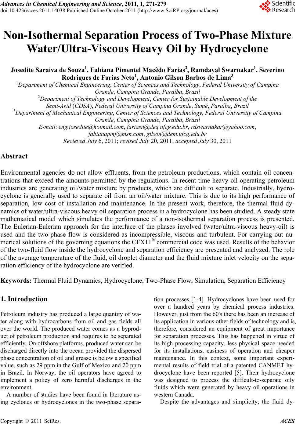
Advances in Chemical Engi neering and Science , 2011, 1, 271-279
doi:10.4236/aces.2011.14038 Published Online October 2011 (http://www.SciRP.org/journal/aces)
Non-Isoth e rma l S epa rat ion Process of Two-Phase Mixture
Water/Ultra-Viscous Heavy Oil by Hydr ocyclone
Josedite Saraiva de Souza1, Fabiana Pimentel Macêdo Farias2, Ramdayal Swarnakar1, Severino
Rodrigues de Farias Neto1, Antonio Gilson Barbos de Lima3
1Department of Chemical Engineering, Center of Sciences and Technology, Federal University of Campina
Grande, Campina Grande, Paraíba, Brazil
2Department of Technology and Development, Center for Sustainable Development of the
Semi-Arid (CDSA), Federal University of Campina Grande, Sumé, Paraíba, Brazil
3Department of Mechanical Engineering, Center of Sciences and Technology, Federal University of Campina
Grande, Campina Grande, Paraíba, Brazil
fabianapmf@m sn.com,
Recieved July 6, 2011; revised July 20, 2011; accepted July 30, 2011
Abstract
Environmental agencies do not allow effluents, from the petroleum productions, which contain oil concen-
trations that exceed the amounts permitted by the regulations. In recent time heavy oil operating petroleum
industries are generating oil/water mixture by products, which are difficult to separate. Industrially, hydro-
cyclone is generally used to separate oil from an oil/water mixture. This is due to its high performance of
separation, low cost of installation and maintenance. In the present work, therefore, the thermal fluid dy-
namics of water/ultra-viscous heavy oil separation process in a hydrocyclone has been studied. A steady state
mathematical model which simulates the performance of a non-isothermal separation process is presented.
The Eulerian-Eulerian approach for the interface of the phases involved (water/ultra-viscous heavy-oil) is
used and the two-phase flow is considered as incompressible, viscous and turbulent. For carrying out nu-
merical solutions of the governing equations the CFX11® commercial code was used. Results of the behavior
of the two-fluid flow inside the hydrocyclone and separation efficiency are presented and analyzed. The role
of the average temperature of the fluid, oil droplet diameter and the fluid mixture inlet velocity on the sepa-
ration efficiency of the hydrocyclone are verified.
Keywords: Thermal Fluid Dynamics, Hydrocyclone, Two-Phase Flow, Simulation, Separation Efficiency
1. Introduction
Petroleum industry has produced a large quantity of wa-
ter along with hydrocarbons from oil and gas fields all
over the world. The produced water comes as a byprod-
uct of petroleum production and requires to be separated
efficiently. On offshore platforms, produced water can be
discharged directly into the ocean provided the dispersed
phase concentration of oil and grease is below a specified
value, such as 29 ppm in the Gulf of Mexico and 20 ppm
in Brazil. In Norway, the oil operators have agreed to
implement a policy of zero harmful discharges in the
environment.
A number of studies have been found in literature us-
ing cyclones or hydrocyclones in the two-phase separa-
tion processes [1-4]. Hydrocyclones have been used for
over a hundred years by chemical process industries.
However, just from the 60's there has been an increase of
its application in various other fields of technology and is,
therefore, considered an equipment of great importance
for separation processes. This has happened in virtue of
its high processing capacity, less physical space needed
for its installations, easiness of operation and cheaper
maintenance. In this context, some important experi-
mental results of field trial of a patented CANMET hy-
drocyclone have been reported [5]. Their hydrocyclone
was designed to process the difficult-to-separate oily
fluids which were generated by heavy oil operations in
western Canada.
Despite the advantages and simplicity, the fluid dy-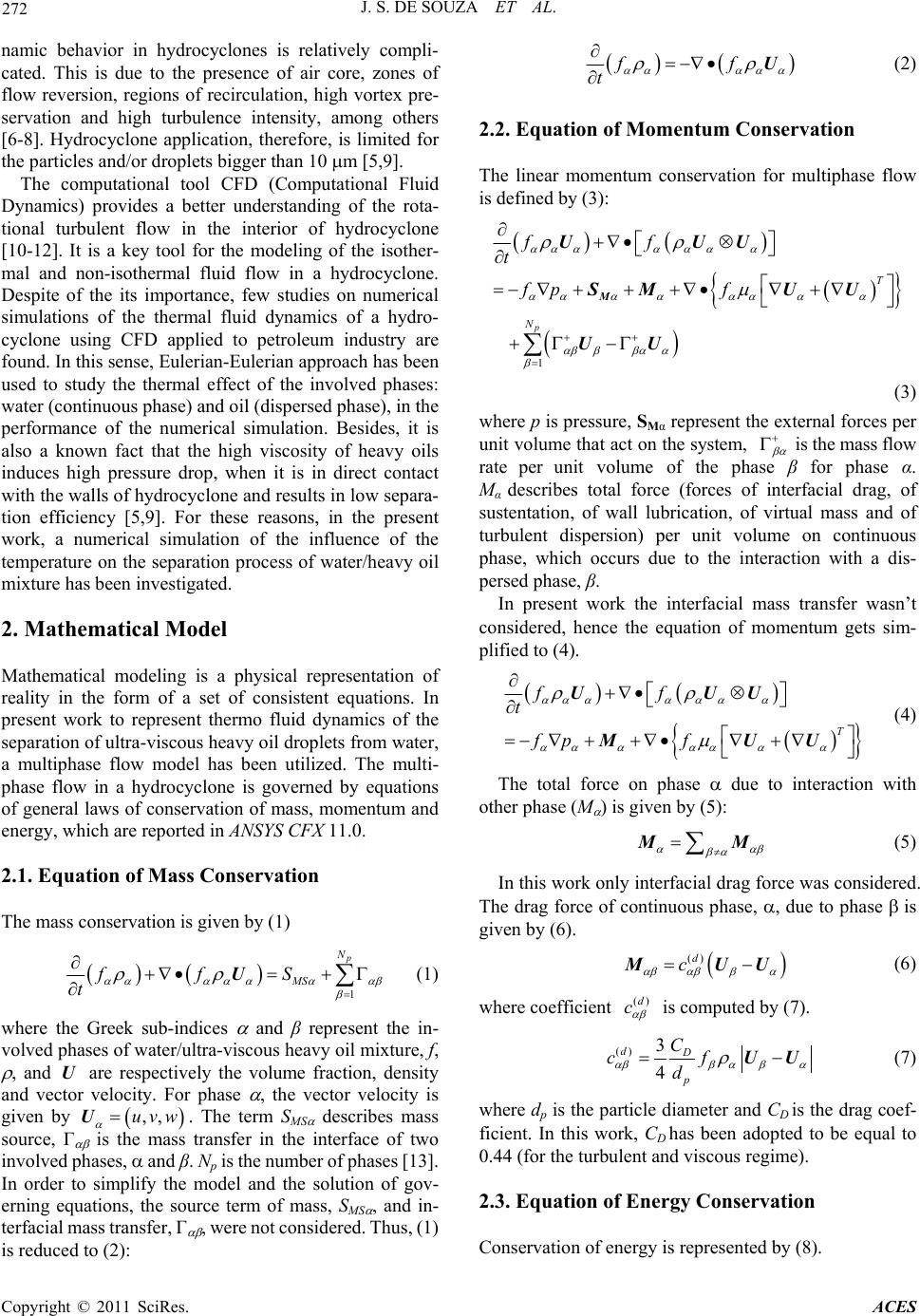

272 J. S. DE SOUZA ET AL.
namic behavior in hydrocyclones is relatively compli-
cated. This is due to the presence of air core, zones of
flow reversion, regions of recirculation, high vortex pre-
servation and high turbulence intensity, among others
[6-8]. Hydrocyclone application, therefore, is limited for
the particles and/or droplets bigger than 10 m [5,9].
The computational tool CFD (Computational Fluid
Dynamics) provides a better understanding of the rota-
tional turbulent flow in the interior of hydrocyclone
[10-12]. It is a key tool for the modeling of the isother-
mal and non-isothermal fluid flow in a hydrocyclone.
Despite of the its importance, few studies on numerical
simulations of the thermal fluid dynamics of a hydro-
cyclone using CFD applied to petroleum industry are
found. In this sense, Eulerian-Eulerian approach has been
used to study the thermal effect of the involved phases:
water (continuous phase) and oil (dispersed phase), in the
performance of the numerical simulation. Besides, it is
also a known fact that the high viscosity of heavy oils
induces high pressure drop, when it is in direct contact
with the walls of hydrocyclone and results in low separa-
tion efficiency [5,9]. For these reasons, in the present
work, a numerical simulation of the influence of the
temperature on the separation process of water/heavy oil
mixture has been investigated.
2. Mathematical Model
Mathematical modeling is a physical representation of
reality in the form of a set of consistent equations. In
present work to represent thermo fluid dynamics of the
separation of ultra-viscous heavy oil droplets from water,
a multiphase flow model has been utilized. The multi-
phase flow in a hydrocyclone is governed by equations
of general laws of conservation of mass, momentum and
energy, which are reported in ANSYS CFX 11.0.
2.1. Equation of Mass Conservation
The mass conservation is given by (1)
 
1
p
N
MS
ffS
t





 

U


(1)
where the Greek sub-indices  and β represent the in-
volved phases of water/ultra-viscous heavy oil mixture, f,
 , and are respectively the volume fraction, density
and vector velocity. For phase
 , the vector velocity is
given by . The term SMS

describes mass
source, Г

is the mass transfer in the interface of two
involved phases,  and β. Np is the number of phases [13].
In order to simplify the model and the solution of gov-
erning equations, the source term of mass, SMS

, and in-
terfacial mass transfer, Г

, were not considered. Thus, (1)
is reduced to (2):
U
U

,,uvw

 
ff
t







U (2)
2.2. Equation of Momentum Conservation
The linear momentum conservation for multiphase flow
is defined by (3):
 



1
p
T
N
ff
t
fp f
  
 
 






 



 

 

M
UUU
SMU U
UU
(3)
where p is pressure, SMα represent the external forces per
unit volume that act on the system, 



is the mass flow
rate per unit volume of the phase β for phase α.
Mα

describes total force (forces of interfacial drag, of
sustentation, of wall lubrication, of virtual mass and of
turbulent dispersion) per unit volume on continuous
phase, which occurs due to the interaction with a dis-
persed phase, β.
In present work the interfacial mass transfer wasn’t
considered, hence the equation of momentum gets sim-
plified to (4).
 


T
ff
t
fp f
  
 



 



 

UUU
MUU
(4)
The total force on phase  due to interaction with
other phase (M

) is given by (5):


 


MM

(5)
In this work only interfacial drag force was considered.
The drag force of continuous phase, , due to phase is
given by (6).

()d
c

 
MUU
(6)
where coefficient ()d c


is computed by (7).
() 3
4

dD
p
C
cf
d


 UU

(7)
where dp is the particle diameter and CD is the drag coef-
ficient. In this work, CD has been adopted to be equal to
0.44 (for the turbulent and viscous regime).
2.3. Equation of Energy Conservation
Conservation of energy is represented by (8).

J. S. DE SOUZA ET AL.
273
 

1
Np
ss
fhf UhT
t
hhQS
  
 





 


 


)
(8)
where hα, Tα and 
α, denote the static enthalpy, tempera-
ture and thermal conductivity of phase α, respectively and
Sα, describes the external sources of heat. The term
(


s
s
hh
 
represents the heat transfer induced by
mass transfer in the interface of the involved phases. In
this work, the term of heat transfer induced by mass
transfer at the interface and the energy source term, Sα,
have not been considered. This means that there is no
chemical reaction in the present separation process. With
these conditions the equation of energy gets transformed
in (9):
 
fh QfhT
t
 


 

U




(9)
where Qα denotes heat transfer at the interface, from one
phase to another phase, given by (10,11,12).



QQ


 
(10)
being
QQ



(11)
and
0
Q


(12)
Heat transfer across a phase boundary is usually
described in terms of an overall heat transfer coefficient
h

, which is the amount of heat energy crossing a unit
area per unit time per unit temperature difference
between the phases. Thus, the rate of heat transfer, Q

,
per unit time across a phase boundary of interfacial area
per unit volume A

, from phase   to phase , is:

QhATT
 
(13)
This may be written in a form analogous to momen-
tum transfer like that:


()

h
QcTT



(14)
where the volumetric heat transfer coefficient, ()h c


, is
modeled using the correlations described below.
() h
chA



(15)
Hence, the interfacial area per unit volume and the
heat transfer coefficient, h
  are required. It is often
convenient to express the heat transfer coefficient in
terms of a dimensionless Nusselt number:
Nu hd





(16)
In the particle model, the thermal conductivity scale,


 is taken to be the thermal conductivity of the
continuous phase (water), and the length scale, d

 is
taken to be the mean diameter of the dispersed phase
(oil). For the convective heat transfer an empirical corre-
lation (Ranz-Marshall) in (16), has been used. It is
available in ANSYS CFX and is based on the theory of
boundary layer for a steady flow, incompressible Newto-
nian fluid and spherical particles.
0.5 0.3
20.6NuRe Pr (17)
where Nu and Re are the Nusselt and Particles Reynolds
numbers. This correlation is valid for 0< Re < 200 and
0< Pr < 250.
The Prandtl number (Pr) is the ratio of the diffusivity
of momentum and thermal diffusivity, defined by (18):
p
C
Pr




(18)
where Cp is the heat capacity and 

 the viscosity of the
continuous phase (water).
2.4. Turbulence Model
Due to complexity of the turbulent fluid flow inside the
hydrocyclone we use k-  model (RNG) to complete the
mathematical formulation. The renormalization group
(RNG) k-
 model is similar in form to the k-  model but
includes additional terms for turbulence dissipation rate
 ,
furnishing more accurate predictions of the flow situa-
tions, including, separation process, streamlines, curves
and stagnant regions.
The values of turbulent kinetic energy, k, and turbulent
dissipation rate, are directly obtained from the differ-
ential equations of transport as can be observed in (19)
and (20):
 
t
k
kRNG
kkP
t

 



k

 
 



U
(19)
 

12
t
RNG kRNG
RNG
t
CPC
k


 








 





U

(20)
where  is the dynamic viscosity,  is the density and 
t
is the turbulent viscosity which is given by (21).

274 J. S. DE SOUZA ET AL.
2
t
k
C



 (21)
where C

is an empirical constant, and the values of the
constants are given by:
0.7179
kNRG NRG
C


  (22)
and
21.68 RNG
C


(23)
13
14.38
1.42 1
RNG
RNG
C











(24)
where,
k
R
NG
P
C

  (25)
In this equation k is the turbulence production due to
viscous and buoyancy forces or shear production of tur-
bulence, which is modeled using (26):
P

T
kt k
PP   UUU b (26)
The term Pkb is the production of buoyancy and is
modelled by (27) as follows:
t
kb
p
P

g


 (27)
where
p

is a constant and is equal to 1.
2.5. Boundary Conditions
The following boundary conditions, for the study of hy-
drocyclone, were used:
1) Inlet conditions [5,9]:
Water
ux = 20.0 and 30.0 m/s
uy = uz = 0.0 m/s
Tinlet = 298.0 K
fw = 0.7
Oil
ux = 20.0 and 30.0 m/s
uy = uz= 0.0 m/s
Tinlet = 298.0 K
fo = 0.3
2) Outlet conditions:
A predefined pressure value 1 atm (p = 101325 Pa)
was adopted at overflow and underflow positions of the
hydrocyclone.
3) Conditions at the wall:
 At internal walls of the hydrocyclone, all speed com-
ponents (ux, u
y, u z), for water and heavy oil phases,
were considered to be null (no slip condition);
 A wall roughness of 0.045 mm in hydrocyclone was
adopted;
 The hydrocyclone wall temperature chosen was Twall
= 673 K.
In Tab le 1 the physical properties relating to the fluids
(water and ultra-viscous heavy oil), used in this study,
are shown. For the dynamic viscosity of the oil as a func-
tion of temperature a numerical fit with experimental
data of [14] was made. It generated an equation which is
presented in the Table 2. The average viscosity of the
heavy oil was calculated by the weighed mean of viscos-
ity as a function of the temperature, for the interval of
298 to 673 K, which are temperatures at inlet, Tmin, and
at wall, Tmax, respectively. Thus, an average value of 1.2
Pa.s was obtained (28 and 29), which is within the range
Table 1. Data used in the simulation. Viscosity, considered
as independent of the temper atur e variation.
Cases foil
ux
(m/s)
dp,oil
(10–3 m)
μoil
(Pa.s)
μwater
(Pa.s)
Twall
(K)
Tinlet
(K)
1a 0.330.0 1.000 0.9466 1.2 673.0298.0
2a 0.330.0 0.800 0.9466 1.2 673.0298.0
3a 0.330.0 0.600 0.9466 1.2 673.0298.0
4a 0.330.0 0.400 0.9466 1.2 673.0298.0
5a 0.330.0 0.200 0.9466 1.2 673.0298.0
6a 0.330.0 0.100 0.9466 1.2 673.0298.0
7a 0.330.0 0.010 0.9466 1.2 673.0298.0
8a 0.330.0 0.001 0.9466 1.2 673.0298.0
9a 0.320.0 1.000 0.9466 1.2 673.0298.0
10a 0.3 20.0 0.800 0.9466 1.2 673.0298.0
11a 0.3 20.0 0.600 0.9466 1.2 673.0298.0
12a 0.3 20.0 0.400 0.9466 1.2 673.0298.0
13a 0.3 20.0 0.200 0.9466 1.2 673.0298.0
14a 0.3 20.0 0.100 0.9466 1.2 673.0298.0
15a 0.3 20.0 0.010 0.9466 1.2 673.0298.0
Table 2. Data used in the simulation. Viscosity as a function
of temperature.
Cases foil ux
(m/s)
dp,oil
(10–3 m)
μoil
(Pa.s)
μwat er
(Pa.s)
Twall
(K)
Tinlet
(K)
1b 0.330.01.000* ** 673.0298.0
2b 0.330.00.800* ** 673.0298.0
3b 0.330.00.600* ** 673.0298.0
4b 0.330.00.400* ** 673.0298.0
5b 0.330.00.200* ** 673.0298.0
6b 0.330.00.100* ** 673.0298.0
7b 0.330.00.010* ** 673.0298.0
8b 0.330.00.001* ** 673.0298.0
9b 0.320.01.000* ** 673.0298.0
10b0.320.00.800* ** 673.0298.0
11b0.320.00.600* ** 673.0298.0
12b0.320.00.400* ** 673.0298.0
13b0.320.00.200* ** 673.0298.0
14b0.320.00.100* ** 673.0298.0
15b0.320.00.010* ** 673.0298.0
*3.1871 exp(–2.3 935Tadm***); **0.0009exp(–2.6890Tadm***);
*** adm max
max min
min
min
(T T)
T=whereT673 K andT298 K
(TT)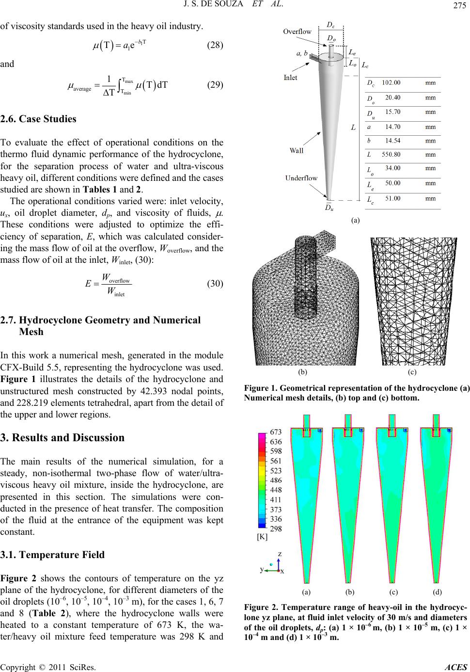

.

J. S. DE SOUZA ET AL.
275
of viscosity standards used in the heavy oil industry.

1T
1
Te
b
a 

 (28)
and

max
min
T
average T
1TdT
T
  (29)
2.6. Case Studies
To evaluate the effect of operational conditions on the
thermo fluid dynamic performance of the hydrocyclone,
for the separation process of water and ultra-viscous
heavy oil, different conditions were defined and the cases
studied are shown in Tables 1 and 2.
The operational conditions varied were: inlet velocity,
ux, oil droplet diameter, dp, and viscosity of fluids,  .
These conditions were adjusted to optimize the effi-
ciency of separation, E, which was calculated consider-
ing the mass flow of oil at the overflow, Woverflow, and the
mass flow of oil at the inlet, Winlet, (30):
overflow
inlet
W
EW  (30)
2.7. Hydrocyclone Geometry and Numerical
Mesh
In this work a numerical mesh, generated in the module
CFX-Build 5.5, representing the hydrocyclone was used.
Figure 1 illustrates the details of the hydrocyclone and
unstructured mesh constructed by 42.393 nodal points,
and 228.219 elements tetrahedral, apart from the detail of
the upper and lower regions.
3. Results and Discussion
The main results of the numerical simulation, for a
steady, non-isothermal two-phase flow of water/ultra-
viscous heavy oil mixture, inside the hydrocyclone, are
presented in this section. The simulations were con-
ducted in the presence of heat transfer. The composition
of the fluid at the entrance of the equipment was kept
constant.
3.1. Temperature Field
Figure 2 shows the contours of temperature on the yz
plane of the hydrocyclone, for different diameters of the
oil droplets (10–6, 10–5, 10–4, 10–3 m), for the cases 1, 6, 7
and 8 (Table 2), where the hydrocyclone walls were
heated to a constant temperature of 673 K, the wa-
ter/heavy oil mixture feed temperature was 298 K and
(a)
(b) (c)
Figure 1. Geometrical representation of the hydrocyclone (a)
Numerical mesh details, (b) top and (c) bottom.
(a) (b) (c) (d)
Figure 2. Temperature range of heavy-oil in the hydrocyc-
lone yz plane, at fluid inlet velocity of 30 m/s and diameters
of the oil droplets, dp: (a) 1 × 10–6 m, (b) 1 × 10–5 m, (c) 1 ×
10–4 m and (d) 1 × 10–3 m.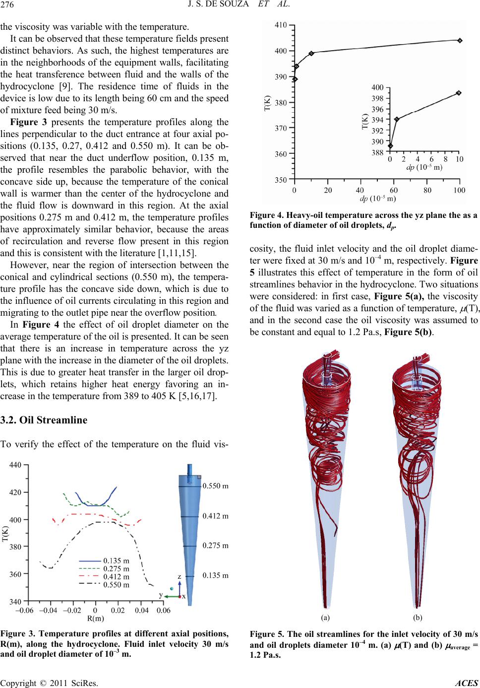

276 J. S. DE SOUZA ET AL.
the viscosity was variable with the temperature.
It can be observed that these temperature fields present
distinct behaviors. As such, the highest temperatures are
in the neighborhoods of the equipment walls, facilitating
the heat transference between fluid and the walls of the
hydrocyclone [9]. The residence time of fluids in the
device is low due to its length being 60 cm and the speed
of mixture feed being 30 m/s.
Figure 3 presents the temperature profiles along the
lines perpendicular to the duct entrance at four axial po-
sitions (0.135, 0.27, 0.412 and 0.550 m). It can be ob-
served that near the duct underflow position, 0.135 m,
the profile resembles the parabolic behavior, with the
concave side up, because the temperature of the conical
wall is warmer than the center of the hydrocyclone and
the fluid flow is downward in this region. At the axial
positions 0.275 m and 0.412 m, the temperature profiles
have approximately similar behavior, because the areas
of recirculation and reverse flow present in this region
and this is consistent with the literature [1,11,15].
However, near the region of intersection between the
conical and cylindrical sections (0.550 m), the tempera-
ture profile has the concave side down, which is due to
the influence of oil currents circulating in this region and
migrating to the outlet pipe near the overflow position.
In Figure 4 the effect of oil droplet diameter on the
average temperature of the oil is presented. It can be seen
that there is an increase in temperature across the yz
plane with the increase in the diameter of the oil droplets.
This is due to greater heat transfer in the larger oil drop-
lets, which retains higher heat energy favoring an in-
crease in the temperature from 389 to 405 K [5,16,17].
3.2. Oil Streamline
To verify the effect of the temperature on the fluid vis-
Figure 3. Temperature profiles at different axial positions,
R(m), along the hydrocyclone. Fluid inlet velocity 30 m/s
and oil droplet diameter of 10–3 m.
Figure 4. Heavy-oil temperature across the yz plane the as a
function of diameter of oil droplets, dp.
cosity, the fluid inlet velocity and the oil droplet diame-
ter were fixed at 30 m/s and 10–4 m, respectively. Figure
5 illustrates this effect of temperature in the form of oil
streamlines behavior in the hydrocyclone. Two situations
were considered: in first case, Figure 5(a), the viscosity
of the fluid was varied as a function of temperature,  (T),
and in the second case the oil viscosity was assumed to
be constant and equal to 1.2 Pa.s, Figure 5(b).
(a) (b)
Figure 5. The oil streamlines for the inlet velocity of 30 m/s
and oil droplets diameter 10–4 m. (a)
 (T) and (b) 
average =
1.2 Pa.s.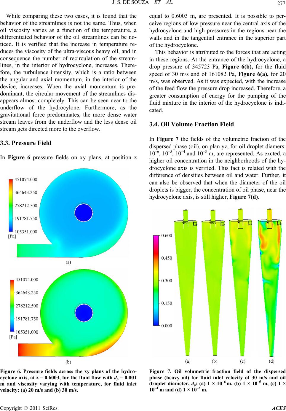

J. S. DE SOUZA ET AL.
277
While comparing these two cases, it is found that the
behavior of the streamlines is not the same. Thus, when
oil viscosity varies as a function of the temperature, a
differentiated behavior of the oil streamlines can be no-
ticed. It is verified that the increase in temperature re-
duces the viscosity of the ultra-viscous heavy oil, and in
consequence the number of recirculation of the stream-
lines, in the interior of hydrocyclone, increases. There-
fore, the turbulence intensity, which is a ratio between
the angular and axial momentum, in the interior of the
device, increases. When the axial momentum is pre-
dominant, the circular movement of the streamlines dis-
appears almost completely. This can be seen near to the
underflow of the hydrocylone. Furthermore, as the
gravitational force predominates, the more dense water
stream leaves from the underflow and the less dense oil
stream gets directed more to the overflow.
3.3. Pressure Field
In Figure 6 pressure fields on xy plans, at position z
(a)
(b)
Figure 6. Pressure fields across the xy plans of the hydro-
cyclone axis, at z = 0.6003, for the fluid flow with dp = 0.001
m and viscosity varying with temperature, for fluid inlet
velocity: (a) 20 m/s and (b) 30 m/s.
equal to 0.6003 m, are presented. It is possible to per-
ceive regions of low pressure near the central axis of the
hydrocyclone and high pressures in the regions near the
walls and in the tangential entrance in the superior part
of the hydrocyclone.
This behavior is attributed to the forces that are acting
in these regions. At the entrance of the hydrocyclone, a
drop pressure of 345723 Pa, Figure 6(b), for the fluid
speed of 30 m/s and of 161082 Pa, Figure 6(a), for 20
m/s, was observed. As it was expected, with the increase
of the feed flow the pressure drop increased. Therefore, a
greater consumption of energy for the pumping of the
fluid mixture in the interior of the hydrocyclone is indi-
cated.
3.4. Oil Volume Fraction Field
In Figure 7 the fields of the volumetric fraction of the
dispersed phase (oil), on plan yz, for oil droplet diamers:
10–6, 10–5, 10–4 and 10–3 m, are represented. As excted, a
higher oil concentration in the neighborhoods of the hy-
drocyclone axis is verified. This fact is related with the
difference of densities between oil and water. Further, it
can also be observed that when the diameter of the oil
droplets is bigger, the concentration of oil phase, near the
hydrocyclone axis, is still higher, Figure 7(d).
(a) (b) (c) (d)
Figure 7. Oil volumetric fraction field of the dispersed
phase (heavy oil) for fluid inlet velocity of 30 m/s and oil
droplet diameter, dp: (a) 1 × 10–6 m, (b) 1 × 10–5 m, (c) 1 ×
10–4 m and (d) 1 × 10–3 m.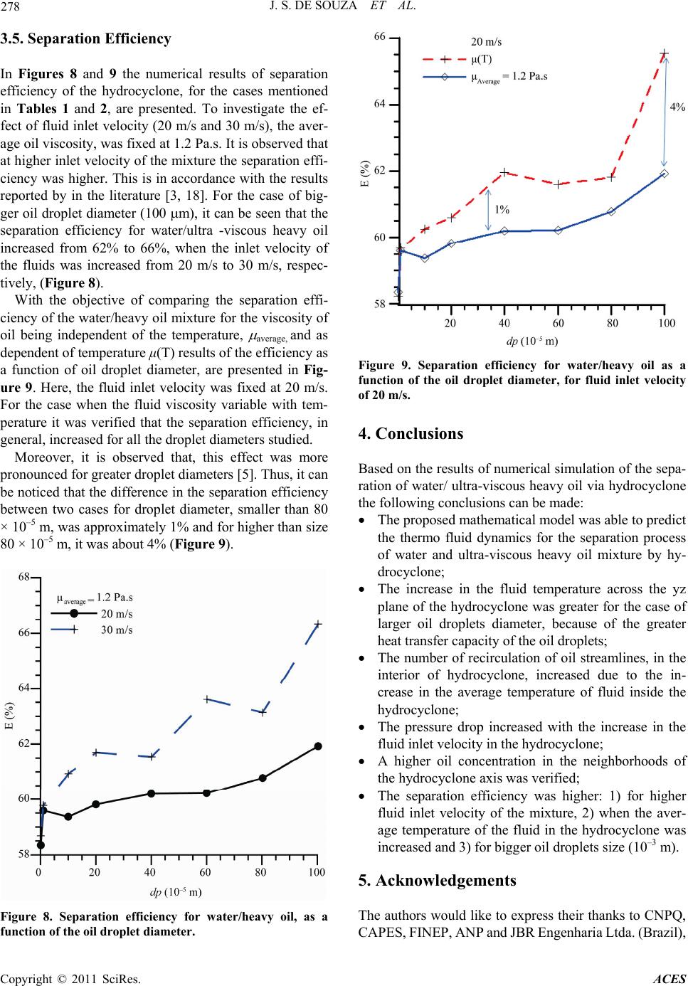

278 J. S. DE SOUZA ET AL.
3.5. Separation Efficiency
In Figures 8 and 9 the numerical results of separation
efficiency of the hydrocyclone, for the cases mentioned
in Tables 1 and 2, are presented. To investigate the ef-
fect of fluid inlet velocity (20 m/s and 30 m/s), the aver-
age oil viscosity, was fixed at 1.2 Pa.s. It is observed that
at higher inlet velocity of the mixture the separation effi-
ciency was higher. This is in accordance with the results
reported by in the literature [3, 18]. For the case of big-
ger oil droplet diameter (100 m), it can be seen that the
separation efficiency for water/ultra -viscous heavy oil
increased from 62% to 66%, when the inlet velocity of
the fluids was increased from 20 m/s to 30 m/s, respec-
tively, (Figure 8).
With the objective of comparing the separation effi-
ciency of the water/heavy oil mixture for the viscosity of
oil being independent of the temperature,

average, and as
dependent of temperature μ(T) results of the efficiency as
a function of oil droplet diameter, are presented in Fig-
ure 9. Here, the fluid inlet velocity was fixed at 20 m/s.
For the case when the fluid viscosity variable with tem-
perature it was verified that the separation efficiency, in
general, increased for all the droplet diameters studied.
Moreover, it is observed that, this effect was more
pronounced for greater droplet diameters [5]. Thus, it can
be noticed that the difference in the separation efficiency
between two cases for droplet diameter, smaller than 80
× 10–5 m, was approximately 1% and for higher than size
80 × 10–5 m, it was about 4% (Figure 9).
Figure 8. Separation efficiency for water/heavy oil, as a
function of the oil droplet diameter.
Figure 9. Separation efficiency for water/heavy oil as a
function of the oil droplet diameter, for fluid inlet velocity
of 20 m/s.
4. Conclusions
Based on the results of numerical simulation of the sepa-
ration of water/ ultra-viscous heavy oil via hydrocyclone
the following conclusions can be made:
 The proposed mathematical model was able to predict
the thermo fluid dynamics for the separation process
of water and ultra-viscous heavy oil mixture by hy-
drocyclone;
 The increase in the fluid temperature across the yz
plane of the hydrocyclone was greater for the case of
larger oil droplets diameter, because of the greater
heat transfer capacity of the oil droplets;
 The number of recirculation of oil streamlines, in the
interior of hydrocyclone, increased due to the in-
crease in the average temperature of fluid inside the
hydrocyclone;
 The pressure drop increased with the increase in the
fluid inlet velocity in the hydrocyclone;
 A higher oil concentration in the neighborhoods of
the hydrocyclone axis was verified;
 The separation efficiency was higher: 1) for higher
fluid inlet velocity of the mixture, 2) when the aver-
age temperature of the fluid in the hydrocyclone was
increased and 3) for bigger oil droplets size (10–3 m).
5. Acknowledgements
The authors would like to express their thanks to CNPQ,
CAPES, FINEP, ANP and JBR Engenharia Ltda. (Brazil),

J. S. DE SOUZA ET AL.
279
for supporting this work, and are also grateful to the au-
thors cited in the text that helped in the improvement of
quality.
6. References
[1] L. Svarovsky, “Solid-Liquid Separation, Chemical Engi-
neering Series,” 4th Edition, Butterworths, London, 2000.
[2] B. Wang and A. B. Yu, “Numerical Study of Particle-
Fluid Flow in Hydrocyclones with Different Body Di-
mensions,” Minerals Engineering, Vol. 19, No. 10, 2006,
pp. 1022-1033. doi:10.1016/j.mineng.2006.03.016
[3] T. Husveg, O. Rambeau, T. Drengstig and T. Bilstad,
“Performance of Deoling Hydrocyclone during Variables
Flow Rates,” Minerals Engineering, Vol. 20, No. 4, 2007,
pp. 368-379. doi:10.1016/j.mineng.2006.12.002
[4] L. G. M. Vieira, J. J. R. Damasceno and M. A. S. Barrozo,
“Improvement of Hydrocyclone Separation Performance
by Incorporating a Conical Filtering Wall,” Chemical
Engineering and Process, Vol. 49, No. 5, 2010, pp. 460-
467. doi:10.1016/j.cep.2010.03.011
[5] K. A. Hashmi, H. A. Hamza and J. C. Wilson, “CAN-
MET Hydrocyclone: An Emerging Alternative for the
Treatment of Oily Waste Streams,” Minerals Engineering,
Vol. 17, No. 5, 2004, pp. 643-649.
doi:10.1016/j.mineng.2004.01.019
[6] V. Krishna, R. Sripriya, V. Kumar, S. Chakraborty and B.
C. Meikap, “Identification and Prediction of Air Core
Diameter in a Hydrocyclone by a Novel Online Sensor
Based on Digital Signal Processing Technique,” Chemi-
cal Engineering and Process, Vol. 49, No. 2, 2010, pp.
165-176. doi:10.1016/j.cep.2010.01.003
[7] M. J. Doby, A. F. Nowakowski, I. Yiu and T. Dyakowski,
“Understanding Air Core Formation in Hydrocyclones by
Studying Pressure Distribution as a Function of Viscos-
ity,” Journal of Mineral Processing, Vol. 86, No. 1-4,
2008, pp. 18-25. doi:10.1016/j.minpro.2007.09.002
[8] P. Bamrungsri, C. Puprasert, C. Guigui, P. Marteil, P.
Bréant and G. Hérbrad, “Development of a Simple Ex-
perimental Method for the Determination of the Liquid
Field Velocity in Conical and Cylindrical Hydrocyc-
lones,” Minerals Engineering Research and Design, Vol.
86, No. 11, 2008, pp. 1263-1270.
[9] J. S. Souza, “Numerical Study of Thermo Fluid Dynamic
Separation of Heavy Oils Oily Waters of a Stream by Hy-
drocyclone,” Master’s Thesis, Federal University of Cam-
pina Grande, Brazil, 2009.
[10] B. Wang, D. L. Xu, G. X. Xiao, W. E. K. Chu and A. B.
Yu, “Numerical Study of Gas-Solid Flow in a Cyclone
Separator,” Third International Conference on CFD in
the Mineral and Process Industrial, Melbourne, 10-12
December 2003, pp. 371-376.
[11] M. Narasimha, M. Brennan and P. N. Holthman, “A Re-
view of CFD Modeling for Performance Predictions of
Hydrocyclone,” Engineering Applications of Computa-
tional Fluid Mechanics, Vol. 1, No. 2, 2007, pp. 109-125.
[12] H. F. Meier and M. Mori, “Gas-Solid Flow in Cyclones:
The Eulerian-Eulerian Approach,” Computers Chemical
Engineering, Vol. 22, Suppl. 1, 1998, pp. S641-S644.
doi:10.1016/S0098-1354(98)00114-8
[13] ANSYS CFX, “User Manual Theory,” USA, 2006.
[14] T. Babadagli and A. Al-Bemani, “Investigations on Ma-
trix Recovery during Steam Injection into Heavy-Oil
Containing Carbonate Rocks,” Journal Petroleum Sci0
ence and Engineering, Vol. 58, No. 1-2, 2007, pp. 259-
274. doi:10.1016/j.petrol.2007.01.003
[15] R. B. Xiang and K. W. Lee, “Numerical Study of Flow
Field in Cyclones of Different Height,” Chemical Engi-
neering and Process, Vol. 44, No. 8, 2005, pp. 877-883.
doi:10.1016/j.cep.2004.09.006
[16] H. Yoshida, T. Takashina, K. Fukuia and T. Iwanaga,
“Effect of Inlet Shape and Slurry Temperature on the
Classification Performance of Hydrocyclones,” Powder
Technology, Vol. 140, No. 1-2, 2004, pp. 1-9.
doi:10.1016/j.powtec.2003.12.006
[17] J. J. Cilliers, L. Diaz-Anadon and F. S. Wee, “Tempera-
ture, Classification and Dewatering in 10 mm Hydro-cy-
clones,” Minerals Engineering, Vol. 17, No. 5, 2004, pp.
591-597. doi:10.1016/j.mineng.2003.11.022
[18] M. A. Bennett and R. A. Williams, “Monitoring the Op-
eration of an Oil/Water Separator Using Impedance To-
mography,” Minerals Engineering, Vol. 17, No. 5, 2004,
pp. 605-614. doi:10.1016/j.mineng.2004.01.021