Journal of Geographic Information System, 2011, 3, 357-366
doi:10.4236/jgis.2011.34034 Published Online October 2011 (http://www.SciRP.org/journal/jgis)
Spatial Monetary Economic Growth with Housing and
Residential Distribution over the Urban Area
Wei-Bin Zhang
Ritsumeikan Asia Pacific University, Beppu-shi, Japan
Received May 26, 2011; revised July 5, 2011; accepted July 20, 2011
Abstract
This study introduces space, transportation, and money into an economic growth model. Growth theory neglects
the importance of transportation on economic growth and transportation economics fails to properly explain how
changes in transportation conditions (such as technological improvement, infrastructure investment, and oil
prices) affect long-term economic growth. By proposing a growth model with transportations, we try to explain
effects of transportation on economic growth. Our model describes dynamic interactions among capital accumu-
lation, travel time, housing, residential distribution, amenity, and endogenous time distribution among work,
travel, and leisure. The study examines effects of inflation policy, transportation conditions, and other conditions
on long-term economic growth and economic geography. The paper demonstrates a way to integrating some
important models in the literature in economic growth theory, urban economics, and transportation research so
that the significance of transportation systems upon economies can be properly analyzed.
Keywords: Economic Growth, Capital Accumulation, Travel Speed, Leisure Time, Housing Rent, Land Rent,
Inflation Policy, CIA Approach
1. Introduction
This study examines effects of transportation conditions
and monetary policy on long-term economic growth.
Although there are many models of economic growth,
there are only a few formal economic growth models
which explicitly introduce transportation conditions into
economic growth theory. Nevertheless, it is obvious that
changes in transportation conditions such as technological
improvement, infrastructure investment and oil price will
affect economic growth. Nevertheless, formal economic
growth theory fails to explain how economic growth is
related to transportation conditions. Another important
issue which is seldom studied in the literature of spatial
economics is how money affects spatial economic growth.
It is well known that relations between economic growth
and money have been extensively analyzed in the literature
of economic growth since Tobin published his seminar
work about growth and money in 1956. Relations between
economic growth and transportation systems with money
have been seldom examined in the literature of theoretical
economics. Money and transportation systems connect
almost all aspects of human interactions across space over
time. As effects of transportation systems and money can
be properly evaluated only over long period of time, a
genuine dynamic approach to interactions, for instance,
between transportation systems and economic development
is required. Theoretical economics lacks a proper analytical
framework for discussing these issues. A main reason for
the omission of studying interactions of economic growth,
money and transportation conditions is that the traditional
economic growth lacks a suitable analytical framework.
The objective of this paper is to study monetary
growth with economic geography and transport systems.
This study is to introduce money into a dynamic model
proposed by Zhang [1]. The model by Zhang deals with
an interaction among capital accumulation, land, housing,
environment, transportation in an isolated linear econ-
omy, by synthesizes the main ideas in the Solow growth
model in the neoclassical growth theory, the Alonso ur-
ban model and the Muth housing model in the urban
economics in an alternative framework to the traditional
neoclassical growth theory. The main difference between
this study and the model by Zhang is that this model in-
troduces money into Zhang’s model with the CIA ap-
proach. The paper is organized as follows. Section 2 de-
fines the basic model. Section 3 guarantees existence of
spatial equilibrium. Section 4 simulates the model with

W.-B. ZHANG 358
the Cobb-Douglas production function. Section 5 exam-
ines effects of change in the inflation policy, CIA pa-
rameter and transportation conditions on the spatial equi-
librium. Section 6 concludes the study. Appendix A
proves the main results in Section 3.
2. The Model
The model is a combination of the basic features of the four
key models, the Solow growth model, the Alonso urban
model, the Muth housing model in the neoclassical growth
theory and urban economics, and the monetary growth
model in the CIA approach. Most “real” aspects of the
model are similar to the model proposed by [1], except that
this study introduces money to the spatial economy. The
monetary aspects of the model with the CIA approach are
examined in a recent book on monetary growth theory by
[2]. As far as urban structures are concerned, we follow the
standard residential land-use model. The basic features of
this model are that an isolated city state is built on a flat
featureless plain. All residents in the economy work in the
CBD. People travel only between their homes and the CBD.
Travel is equally costly in terms of time and money in all
directions. An individual may reside at only one location.
The only spatial characteristic of any location that directly
matters is the distance from the city center. The population
is homogenous. The households achieve the same utility
level regardless of where they locate. All the markets are
perfectly competitive. The system is geographically linear
and consists of two parts - the CBD and the residential area.
The isolated state consists of a finite strip of land with fixed
(territory) length, , extending from the CBD with
constant unit width. We assume that all economic activities
are concentrated in the CBD. The households occupy the
residential area. We assume that the CBD is located at the
left-side end of the linear territory. As we will get the same
conclusions if we locate the CBD at the center of the linear
system, the specified urban configuration will not affect
our discussion.
L
The system consists of industrial and housing sectors.
The industrial production is the same as that in the
one-sector neoclassical growth model. We assume that the
industrial product can be either invested or consumed. The
housing production is similar to that in the Muth model.
Housing is supplied with combination of capital and land.
We assume that the total labor force is fully employed by
the industrial sector. We select industrial good to serve as
numeraire. As we assume that the transportation cost of
workers to the CBD is dependent on the travel distance,
land rent for housing should be spatially different. Let
and
N

Nt respectively stand for fixed population and the
total labor input at time . We assume that industrial
production is carried out by combination of capital and
labor force in the form of
t
  
,
i
F
Kt Nt, where


i
K
t
is capital stocks employed by the industrial sector. Assume
F
to be neoclassical [3]. Introduce /.N
ii
kK We
have




,,1 .
i
ii
FK N
fk Fk
N

The function,


,
i
f
k has the following properties: 1)


00f;

2)


i
f
k is increasing, strictly concave on
,R

and on
2
C;R

 and

'
i
fk0


"0
i
fk ;

and 3)


'fk
0
i
ki
lim

 and

'fklim 0.
i
ki

Markets are competitive; thus labor and capital earn their
marginal products, and firms earn zero profits. The rate of
interest,


,rt and wage rates, are determined by
markets. Hence, for any individual firm and

,wt

rt


wt
are given at each point of time. The production sector
chooses the two variables,

i
K
t and


,Nt to
maximize its profit. The marginal conditions are given by


', '
ki ii
rfkwfkkf   

,
i
k (1)
where k

is the depreciation rate of physical capital.
We now describe housing production and behavior of
households. We us

to denote distance from the CBD to
a point in the residential area. The total labor input,


,Nt
is the sum of the labor input over the space. Let


,Tt 
and


,
h
T  t respectively stand for work time and leisure
time of a household at location ,

and


t,  n and


,Lt 
h respectively for the residential density and lot
size of a household at location .

According to the
definitions of


,,nt 


,T  t and

,Nt we have
 
0
,,d.

 
L
 Ntn tTt

t
(2)
Residential housing assets play a dual in the economy.
First, residential housing assets are used as a durable
consumption good. They are the source of housing services.
Residential housing assets are used as a mechanism for the
intertemporal transfer of wealth, which generates both rents
and capital gains through housing appreciation. It is well
known that Muth introduces a commodity “housing” rather
than land in describing dwelling conditions. Housing is
produced with land and non-land inputs. Households have
a derived demand for land, dependent on both preferences
for housing and technical characteristics of housing
production function. We follow this approach in explaining
decision making of dwelling sites of households. The
housing industry supplies housing services by combining
land and capital. Let us denote housing service
received by the household at location

,
h
c 
.

We specify the
housing service production function as follows






,,,, 1,,
hh
hhh hhhh
ctktL t

 0,

 
(3)
where (,)
h
kt

is the input level of capital per household
C
opyright © 2011 SciRes. JGIS

W.-B. ZHANG359
at location,

. Here, we assume that housing capital can
be instantaneously adjusted. All the characteristics of
houses such as the size of a lot and the size of a house can
be changed instantaneously without costs. Hence the
capital-land ratio is always perfectly adjusted. It should be
note that our approach is mainly based on [4]. The Anas
housing production includes the labor input. Further
issues related to the durability of real estates and its
costly conversion and replacements are also discussed in
[4]. See also [5-8] for introducing more realistic aspects
of housing market to the growth model. A recent
literature review is referred to [9].
Let and stand for respectively the
land rent and housing rent at

,
 
tRt 

,
h
R 
.

The marginal conditions
are given by
,,0
hhh hhh
k
hh
Rc Rc
rR
kL


. L

  (4)
According to the definitions of and we have
h
L,n
1
(,),0 .
(,)
h
nt L
Lt


 (5)
The total capital stocks employed by the housing sector
is equal to the sum of the capital stocks for housing over
space at any point of time.
The relationship between


,
h
k  t and the total capital
stocks employed by the housing sector,

,
h
K
t is given
by
 
0
,,
L
hh
.
K
tntktd

   (6)
Each worker may get income from land ownership,
wealth ownership and wages. In order to define incomes, it
is necessary to determine land ownership structure. It can
be seen that land properties may be distributed in multiple
ways under various institutions. There are three
often-applied assumptions in the literature of urban
economics. They are the absentee landownership, the
public ownership, and the equally shared landownership.
The absentee landownership assumption means that land
is owned by absentee landlords who spend their land
incomes outside the economic system. This may also be
interpreted as that the government spends the income
from land on public goods such as military and
households equally benefit from the public goods. If the
public goods enter the utility in the following way,
 
H
gUx where

H
g is a function of the public
goods,
g
being independent of location and
x
is the
vector of the other factors that affect the utility, the
model is mathematically identical to the interpretation
just described. In the case of the public ownership, for
instance as accepted in [10], the city government rents
the land from the landowners at certain rent and sublets it
to households at the market rent, using the net revenue to
subsidize city residents equally. The equally shared
landownership means that the land is equally shared by
the population and the income from the land is equally
shared among the population. To simplify the model, we
assume the absentee landownership. This means that the
income from land rent is spent outside the economic
system.
We assume that agents have perfect foresight with
respect to all future events and capital markets operate
frictionless. The government levies no taxes. Money is
introduced by assuming that a central bank distributes at no
cost to the population a per capita amount of fiat money


0.Mt  The government may distribute the money in
various ways and there are different mechanisms for the
government to issue money. As systematically
demonstrated in [2], it is possible to build the model
according to specified characters of the monetary system.
The scheme according to which the money stock evolves
over time is deterministic and known to all agents. With

being the constant net growth rate of the money stock,


M
t evolves over time according:


,0Mt Mt  .



At the government brings t


M
t  additional units
of money per capita into circulation in order to finance all
government expenditures via seigniorage. Let


mt stand
for the real value of money per capita measured in units of
the output good, that is,
 


/Pt.mt Mt The
government expenditure in real terms per capita,


,t  is
given by





 
.
Mt Mt
tm
Pt Pt


 

t
The representative household receives units of
paper money from the government through a “helicopter
drop”, also considered to be independent of his money
holdings. Consumers make decisions on choice of lot size,
consumption level of commodity as well as on how much
to save. Let

mt 


,mt  and stand for
respectively the per capita real money balances and wealth
(excluding land) owned by the typical household in at
location

k 

,t
.

Each household at

obtains the real
income










  
,, ,
π,, 0
 
 

.


ytrtktwtTt
tm tmtL
(7)
The disposable income is given by




ˆ,,,,
y
ty tat   (8)
where




,,atktmt   ,.
At each point of
time, a consumer at location

distributes the total
available income among holding money,


,,mt 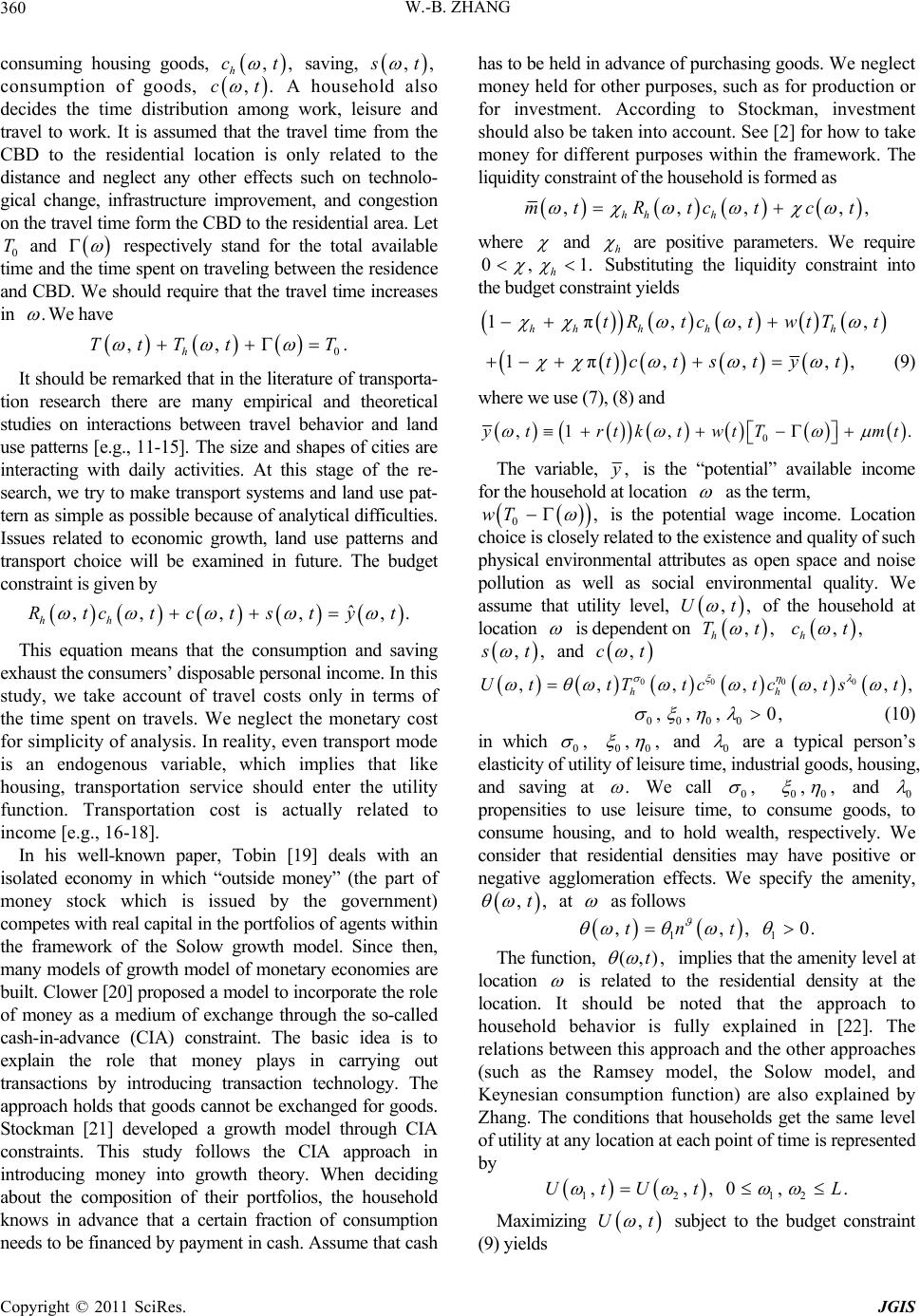

W.-B. ZHANG 360
consuming housing goods,


,,
h
ct  saving,


,,
s
t 
consumption of goods,


,.ct  A household also
decides the time distribution among work, leisure and
travel to work. It is assumed that the travel time from the
CBD to the residential location is only related to the
distance and neglect any other effects such on technolo-
gical change, infrastructure improvement, and congestion
on the travel time form the CBD to the residential area. Let
0 and T



 respectively stand for the total available
time and the time spent on traveling between the residence
and CBD. We should require that the travel time increases
in .

We have
 
0h
TtT T  

c

,,t

,ts  
.

,.yt  
It should be remarked that in the literature of transporta-
tion research there are many empirical and theoretical
studies on interactions between travel behavior and land
use patterns [e.g., 11-15]. The size and shapes of cities are
interacting with daily activities. At this stage of the re-
search, we try to make transport systems and land use pat-
tern as simple as possible because of analytical difficulties.
Issues related to economic growth, land use patterns and
transport choice will be examined in future. The budget
constraint is given by
 
ˆ
,, ,
hh
Rtct t  
This equation means that the consumption and saving
exhaust the consumers’ disposable personal income. In this
study, we take account of travel costs only in terms of
the time spent on travels. We neglect the monetary cost
for simplicity of analysis. In reality, even transport mode
is an endogenous variable, which implies that like
housing, transportation service should enter the utility
function. Transportation cost is actually related to
income [e.g., 16-18].
In his well-known paper, Tobin [19] deals with an
isolated economy in which “outside money” (the part of
money stock which is issued by the government)
competes with real capital in the portfolios of agents within
the framework of the Solow growth model. Since then,
many models of growth model of monetary economies are
built. Clower [20] proposed a model to incorporate the role
of money as a medium of exchange through the so-called
cash-in-advance (CIA) constraint. The basic idea is to
explain the role that money plays in carrying out
transactions by introducing transaction technology. The
approach holds that goods cannot be exchanged for goods.
Stockman [21] developed a growth model through CIA
constraints. This study follows the CIA approach in
introducing money into growth theory. When deciding
about the composition of their portfolios, the household
knows in advance that a certain fraction of consumption
needs to be financed by payment in cash. Assume that cash
has to be held in advance of purchasing goods. We neglect
money held for other purposes, such as for production or
for investment. According to Stockman, investment
should also be taken into account. See [2] for how to take
money for different purposes within the framework. The
liquidity constraint of the household is formed as



  
,,,
hh h
mtR tc tct   ,,
where

and h

are positive parameters. We require
h
0, 1.



 Substituting the liquidity constraint into
the budget constraint yields





 


1π,, ,    
hh hhh
tRtct wtTt





 
1π,,    tctstyt,,
(9)
where we use (7), (8) and














0
,1 ,yt rtktwtTmt    

. 
The variable, ,
y
is the “potential” available income
for the household at location

as the term,




0,wT
  is the potential wage income. Location
choice is closely related to the existence and quality of such
physical environmental attributes as open space and noise
pollution as well as social environmental quality. We
assume that utility level,


,,tU  of the household at
location

is dependent on


,,
h
Tt 

,,
h
ct 


,,
s
t  and


,ct 












0000
,,,,,
hh
U ttTtctctst

   ,,
,

0000
,,, 0

  (10)
in which 0,

00 ,,

and 0

are a typical person’s
elasticity of utility of leisure time, industrial goods, housing,
and saving at .

We call 0,

00 ,,

and 0

propensities to use leisure time, to consume goods, to
consume housing, and to hold wealth, respectively. We
consider that residential densities may have positive or
negative agglomeration effects. We specify the amenity,


,t  , at

as follows


11
,tn

 ,  ,  0.t 


The function, (,),t

 implies that the amenity level at
location

is related to the residential density at the
location. It should be noted that the approach to
household behavior is fully explained in [22]. The
relations between this approach and the other approaches
(such as the Ramsey model, the Solow model, and
Keynesian consumption function) are also explained by
Zhang. The conditions that households get the same level
of utility at any location at each point of time is represented
by




12 12
,,,0,UtU t   .L


Maximizing


,Ut  subject to the budget constraint
(9) yields
C
opyright © 2011 SciRes. JGIS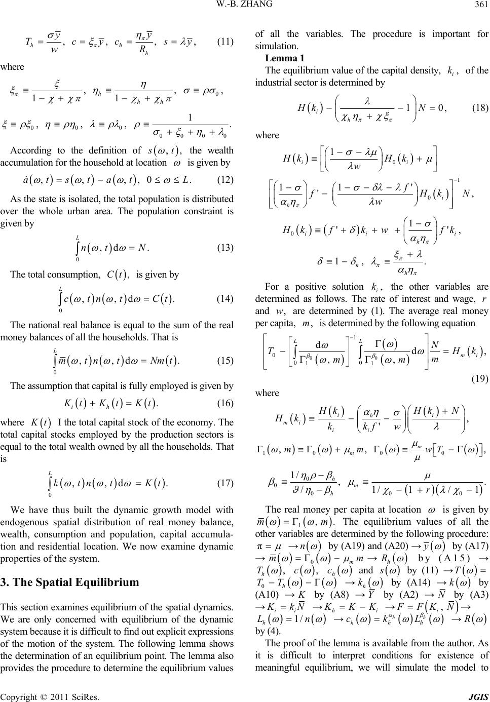

W.-B. ZHANG361
,, ,
hh
h
y
y
Tcycs
wR




, y

   (11)
where
0
,,
11
h
hh


,




 


000
0000
1
,,,

.




According to the definition of

,,
s
t  the wealth
accumulation for the household at location

is given by

,,,,0atstat L    
.
.

.
(12)
As the state is isolated, the total population is distributed
over the whole urban area. The population constraint is
given by

0
,d  

L
nt N
(13)
The total consumption, is given by

,Ct
 
0
,,d  

L
ctnt Ct (14)
The national real balance is equal to the sum of the real
money balances of all the households. That is
 
0
,,d  

L
mtnt Nmt. (15)
The assumption that capital is fully employed is given by
 
.
ih
K
tKtKt (16)
where

K
t I the total capital stock of the economy. The
total capital stocks employed by the production sectors is
equal to the total wealth owned by all the households. That
is
 
0
,,d  

L
ktntKt

. (17)
We have thus built the dynamic growth model with
endogenous spatial distribution of real money balance,
wealth, consumption and population, capital accumula-
tion and residential location. We now examine dynamic
properties of the system.
3. The Spatial Equilibrium
This section examines equilibrium of the spatial dynamics.
We are only concerned with equilibrium of the dynamic
system because it is difficult to find out explicit expressions
of the motion of the system. The following lemma shows
the determination of an equilibrium point. The lemma also
provides the procedure to determine the equilibrium values
of all the variables. The procedure is important for
simulation.
Lemma 1
The equilibrium value of the capital density, of the
industrial sector is determined by
,
i
k

1
i
h
Hk N


 

0,






(18)
where
 

0
1
0
1
11 '
',
ii
i
h
HkH k
w
f
f
Hk N
w

 


 

 


 













 
0
1
''
ii
h
,
i
H
kf kwfk





 


1,
k
h



.





 
For a positive solution the other variables are
determined as follows. The rate of interest and wage,
and are determined by (1). The average real money
per capita, is determined by the following equation
,
i
k
r
,w
,m




00
1
0
00 11
dd,
,,











 




LL
mi
N
TH
m mm k
(19)
where



,
'
ii
h
mi
ii
H
kHk
Hk kkfw
 

 


 



 
N

1000
,,
m
m
mmwT






, 


0
0
00
1/ ,.
/1/1/
h
m
hr
 

 



0
1 
The real money per capita at location

is given by




1,m
  .m The equilibrium values of all the
other variables are determined by the following procedure:
π


→


n

by (A19) and (A20) →

y


by (A17)
→




m
 
0
m   m

h
R→

by (A15) →


,
h
T



,c



ch

and

s

by (11) →


T 





0h
TT

  →


h
k

by (A14) →


k

by
(A10) → by (A8) →
KY by (A2) →N by (A3)
→ii
K
kN →hi
K
KK

 →

,
i
F
FKN→




1/Ln
h

  →


hh
ck


hh
h
L



  →


R

by (4).
The proof of the lemma is available from the author. As
it is difficult to interpret conditions for existence of
meaningful equilibrium, we will simulate the model to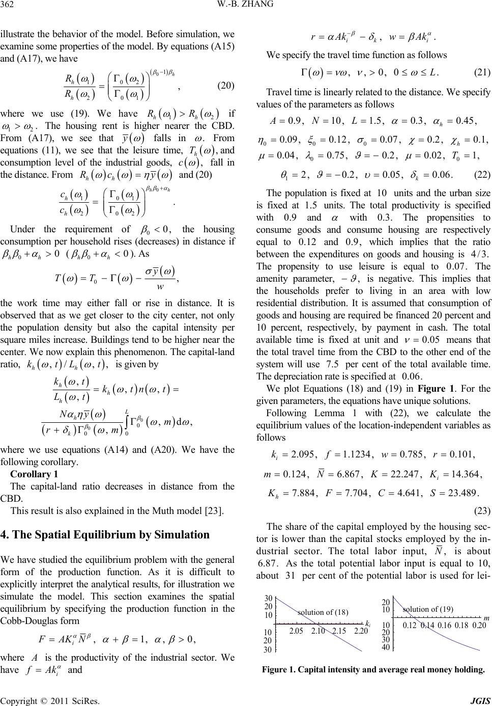

W.-B. ZHANG 362
illustrate the behavior of the model. Before simulation, we
examine some properties of the model. By equations (A15)
and (A17), we have





01
102
201
,
h
h
h
R
R










(20)
where we use (19). We have



12hh
RR

  if
12
.

  The housing rent is higher nearer the CBD.
From (A17), we see that


y

falls in .

From
equations (11), we see that the leisure time,


,
h
T

and
consumption level of the industrial goods,

,c

fall in
the distance. From
 
hh
Rcy

  and (20)




0
101
202
.
hh
h
h
c
c
  








Under the requirement of 00,

 the housing
consumption per household rises (decreases) in distance if
00 hh

  (00
hh

 ). As
 
0,
y
TT w



 
the work time may either fall or rise in distance. It is
observed that as we get closer to the city center, not only
the population density but also the capital intensity per
square miles increase. Buildings tend to be higher near the
center. We now explain this phenomenon. The capital-land
ratio, is given by

,/ ,,
hh
ktLt 

 

 
0
00
0
0
,,,
,
,d
,




 
,





 
h
h
h
L
h
k
kt
ktnt
Lt
Ny m
rm
where we use equations (A14) and (A20). We have the
following corollary.
Corollary 1
The capital-land ratio decreases in distance from the
CBD.
This result is also explained in the Muth model [23].
4. The Spatial Equilibrium by Simulation
We have studied the equilibrium problem with the general
form of the production function. As it is difficult to
explicitly interpret the analytical results, for illustration we
simulate the model. This section examines the spatial
equilibrium by specifying the production function in the
Cobb-Douglas form
,1,,
i
FAKN

  0,
where
A
is the productivity of the industrial sector. We
have i
f
Ak

 and
,.
iki
rAk wAk





We specify the travel time function as follows


,,0,0L   .

 (21)
Travel time is linearly related to the distance. We specify
values of the parameters as follows
0.9,10, 1.5,0.3,0.45,
h
ANL



 
00 0
00
0.09,0.12,0.07, 0.2,0.1,
0.04,0.75,0.2, 0.02,1,
h
T
 
 
 

12,0.2, 0.05,0.06. k



 (22)
The population is fixed at units and the urban size
is fixed at 1 units. The total productivity is specified
with and
10
5.
9.0

with The propensities to
consume goods and consume housing are respectively
equal to 0 and which implies that the ratio
between the expenditures on goods and housing is
The propensity to use leisure is equal to The
amenity parameter,
.3.0
12. ,9.0
,
.3/4
.07.0


is negative. This implies that
the households prefer to living in an area with low
residential distribution. It is assumed that consumption of
goods and housing are required be financed 20 percent and
10 percent, respectively, by payment in cash. The total
available time is fixed at unit and 0.05


.06.0
means that
the total travel time from the CBD to the other end of the
system will use per cent of the total available time.
The depreciation rate is specified at
5.7
We plot Equations (18) and (19) in Figure 1. For the
given parameters, the equations have unique solutions.
Following Lemma 1 with (22), we calculate the
equilibrium values of the location-independent variables as
follows
2.095,1.1234,0.785, 0.101,
i
kf wr


0.124, 6.867, 22.247,14.364,
i
mNK K 
7.884,7.704,4.641, 23.489
h
KFCS.


(23)
The share of the capital employed by the housing sec-
tor is lower than the capital stocks employed by the in-
dustrial sector. The total labor input, ,N is about
As the total potential labor input is equal to 10,
about per cent of the potential labor is used for lei-
.87.6
31
2.052.102.152.20
30
20
10
10
20
30
0.120.14 0.16 0.180.20
40
30
20
10
10
20
solution of (19)
solution of (18) m
ki
Figure 1. Capital intensit y and average real m oney hold ing.
C
opyright © 2011 SciRes. JGIS

W.-B. ZHANG 363
sure and travel. Here, the “potential labor input” is the
labor input if all workers spend all their available time on
working without traveling and enjoying leisure. In this
study, we neglect other possible relations between work
time and work efficiency. The rate of interest is about 7.9
percent. We now plot the equilibrium values of the loca-
tion-dependent variables as in Figure 2. The residential
density, consumption of goods, physical wealt per capita
and real money per capita decline in distance. Both the
housing rent and land rent fall and amenity rises in dis-
tance. The consumption of housing and work time rises
in distance. As the resident lives further away from the
CBD, the leisure time falls.
5. Changes in the Inflation Policy, CIA
Parameter and Transportation
The previous sector shows the equilibrium structure of the
economic geography. We now examine effects of change
in the inflation policy parameter, ,

on the equilibrium.
Let a variable
x
 stand for the change rate of the variable
x
in percentage due to changes in value of a parameter
value. Suppose that the government increases its inflation
policy, ,

from to We represent the
effects in (24) and Figure 3. As it is well known that in
the traditional CIA models the role of money as facilitator
of transactions is reflected in the rule that no transactions
can take place unless the money needed for the transaction
is held for some time in advance. We see that money is not
neutral in the long term, as demonstrated in (24) and Figure
3. We note that although a rise in the growth rate of money
reduces the total capital stock and capital stocks employed
by the two sectors, the output of goods is increased. As
people’s income fall, they tend to work longer hours so that
the total labor input is increased. From Equations (11), we
see that a rise in the growth rate of money implies that the
real price of consumption goods and real housing rent are
increased. As the prices rise, the demand for goods and
housing tend to fall, which would reduce the output levels.
As wage falls and rate of interest rises, people tend to have
lower income, which make people to work longer hours.
People in all the location have more leisure time. The
residential density falls nearer the CBD but increases far
away from the CBD. As a consequence of the residential
redistribution over space, some people reduce their work
hours but some increase their work hours. As a net result,
the total labor input is increased. As the inflation rate
becomes higher, people at any location reduces their 04.0 .05.0
0.20.4 0.6 0.81.01.2 1.4
6.5
7.0
7.5
0.20.40.6 0.8 1.01.2 1.4
0.20
0.25
0.20.40.60.81.01.21.4
0.4
0.5
0.6
0.7
0.8
0.9
k
Th
c
n ωc
ωω
m
0.20.4 0.60.8 1.01.2 1.4
1.0
1.5
2.0
2.5
0.20.40.6 0.81.0 1.21.4
0.74
0.75
0.76
0.77
0.20.4 0.6 0.8 1.0 1.21.4
1.6
1.8
2.0
2.2
2.4
s
T
R θ k
Rωω
ω
Figure 2. The location-dependent variables.
0.20.40.60.81.01.21.4
0.02
0.01
0.01
0.02
0.20.4 0.60.81.0 1.21.4
0.05
0.10
0.15
0.20
0.25
0.20.40.60.81.01.21.4
0.04
0.03
0.02
0.01
ΔThΔch
Δn
ω Δ
k
h
Δm Δc ω
ω
0.20.4 0.60.8 1.01.2 1.4
0.02
0.04
0.06
0.08
0.10
0.12
0.20.40.60.81.01.21.4
0.106
0.104
0.103
0.102
0.101
0.20.40.60.81.01.21.4
0.205
0.210
0.215
0.220
ΔRh
Δk
ΔR ΔT Δs
ω
Δθ ω
ω
Figure 3. The inflation rate and spatial equilibrium.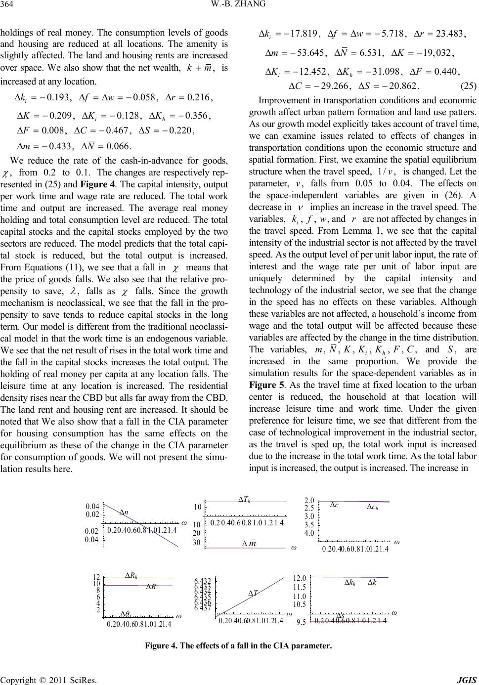

W.-B. ZHANG 364
holdings of real money. The consumption levels of goods
and housing are reduced at all locations. The amenity is
slightly affected. The land and housing rents are increased
over space. We also show that the net wealth, ,km

is
increased at any location.
0.193,0.058, 0.216,
i
kfwr 
0.209, 0.128,0.356,
0.008,0.467, 0.220,
0.433, 0.066.
ih
KK K
FC S
mN
 
 

We reduce the rate of the cash-in-advance for goods,
,

from to The changes are respectively rep-
resented in (25) and Figure 4. The capital intensity, output
per work time and wage rate are reduced. The total work
time and output are increased. The average real money
holding and total consumption level are reduced. The total
capital stocks and the capital stocks employed by the two
sectors are reduced. The model predicts that the total capi-
tal stock is reduced, but the total output is increased.
From Equations (11), we see that a fall in
2.0 .1.0

means that
the price of goods falls. We also see that the relative pro-
pensity to save, ,

falls as

falls. Since the growth
mechanism is neoclassical, we see that the fall in the pro-
pensity to save tends to reduce capital stocks in the long
term. Our model is different from the traditional neoclassi-
cal model in that the work time is an endogenous variable.
We see that the net result of rises in the total work time and
the fall in the capital stocks increases the total output. The
holding of real money per capita at any location falls. The
leisure time at any location is increased. The residential
density rises near the CBD but alls far away from the CBD.
The land rent and housing rent are increased. It should be
noted that We also show that a fall in the CIA parameter
for housing consumption has the same effects on the
equilibrium as these of the change in the CIA parameter
for consumption of goods. We will not present the simu-
lation results here.
17.819,5.718, 23.483,
i
kfwr

 
53.645, 6.531,19,032,
12.452,31.098, 0.440,
ih
mNK
KK F
 

29.266, 20.862.CS

  (25)
Improvement in transportation conditions and economic
growth affect urban pattern formation and land use patters.
As our growth model explicitly takes account of travel time,
we can examine issues related to effects of changes in
transportation conditions upon the economic structure and
spatial formation. First, we examine the spatial equilibrium
structure when the travel speed, is changed. Let the
parameter, falls from to The effects on
the space-independent variables are given in (26). A
decrease in
1/ ,v
.0,v05.0 .04

implies an increase in the travel speed. The
variables, and are not affected by changes in
the travel speed. From Lemma 1, we see that the capital
intensity of the industrial sector is not affected by the travel
speed. As the output level of per unit labor input, the rate of
interest and the wage rate per unit of labor input are
uniquely determined by the capital intensity and
technology of the industrial sector, we see that the change
in the speed has no effects on these variables. Although
these variables are not affected, a household’s income from
wage and the total output will be affected because these
variables are affected by the change in the time distribution.
The variables,
,,,w
i
kf r
,,,K, ,K F,C,
ih and are
increased in the same proportion. We provide the
simulation results for the space-dependent variables as in
Figure 5. As the travel time at fixed location to the urban
center is reduced, the household at that location will
increase leisure time and work time. Under the given
preference for leisure time, we see that different from the
case of technological improvement in the industrial sector,
as the travel is sped up, the total work input is increased
due to the increase in the total work time. As the total labor
input is increased, the output is increased. The increase in
mNK ,S
0.20.40.60.81.01.21.4
0.04
0.02
0.02
0.04
0.20.40.60.8 1.01.21.4
30
20
10
10
0.20.40.60.81.01.21.4
4.0
3.5
3.0
2.5
2.0
ΔThΔcΔch
Δn
ω
Δm ω
ω
0.20.40.60.81.01.21.4
2
4
6
8
10
12
0.20.40.60.81.01.21.4
6.437
6.436
6.435
6.434
6.433
6.432
0.20.4 0.60.81.0 1.2 1.4
9.5
10.5
11.0
11.5
12.0
ΔRh
ΔkhΔk
ΔR ΔT
ω
Δθ ωΔs
ω
Figure 4. The effects of a fall in the CIA parameter.
C
opyright © 2011 SciRes. JGIS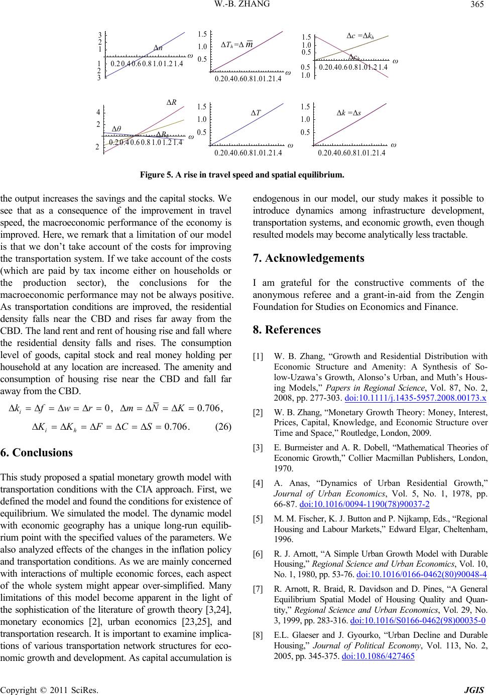

W.-B. ZHANG365
0.2 0.40.6 0.81.0 1.21.4
3
2
1
1
2
3
0.20.40.60.81.01.21.4
0.5
1.0
1.5
0.20.40.60.81.01.21.4
1.0
0.5
0.5
1.0
1.5
Δc =Δkh
Δ
T
h=Δm
Δn
ωΔch ω
ω
0.20.4 0.6 0.8 1.0 1.2 1.4
2
2
4
0.20.40.60.81.01.21.4
0.5
1.0
1.5
0.20.40.60.81.01.21.4
0.5
1.0
1.5
ΔR
ΔTΔk =Δs
ΔθΔRh ω
ω
ω
Figure 5. A rise in travel sp eed and sp atial equilibrium.
the output increases the savings and the capital stocks. We
see that as a consequence of the improvement in travel
speed, the macroeconomic performance of the economy is
improved. Here, we remark that a limitation of our model
is that we don’t take account of the costs for improving
the transportation system. If we take account of the costs
(which are paid by tax income either on households or
the production sector), the conclusions for the
macroeconomic performance may not be always positive.
As transportation conditions are improved, the residential
density falls near the CBD and rises far away from the
CBD. The land rent and rent of housing rise and fall where
the residential density falls and rises. The consumption
level of goods, capital stock and real money holding per
household at any location are increased. The amenity and
consumption of housing rise near the CBD and fall far
away from the CBD.
0, 0.706,
i
kfwr mNK 
0.706.
ih
KK FCS (26)
6. Conclusions
This study proposed a spatial monetary growth model with
transportation conditions with the CIA approach. First, we
defined the model and found the conditions for existence of
equilibrium. We simulated the model. The dynamic model
with economic geography has a unique long-run equilib-
rium point with the specified values of the parameters. We
also analyzed effects of the changes in the inflation policy
and transportation conditions. As we are mainly concerned
with interactions of multiple economic forces, each aspect
of the whole system might appear over-simplified. Many
limitations of this model become apparent in the light of
the sophistication of the literature of growth theory [3,24],
monetary economics [2], urban economics [23,25], and
transportation research. It is important to examine implica-
tions of various transportation network structures for eco-
nomic growth and development. As capital accumulation is
endogenous in our model, our study makes it possible to
introduce dynamics among infrastructure development,
transportation systems, and economic growth, even though
resulted models may become analytically less tractable.
7. Acknowledgements
I am grateful for the constructive comments of the
anonymous referee and a grant-in-aid from the Zengin
Foundation for Studies on Economics and Finance.
8. References
[1] W. B. Zhang, “Growth and Residential Distribution with
Economic Structure and Amenity: A Synthesis of So-
low-Uzawa’s Growth, Alonso’s Urban, and Muth’s Hous-
ing Models,” Papers in Regional Science, Vol. 87, No. 2,
2008, pp. 277-303. doi:10.1111/j.1435-5957.2008.00173.x
[2] W. B. Zhang, “Monetary Growth Theory: Money, Interest,
Prices, Capital, Knowledge, and Economic Structure over
Time and Space,” Routledge, London, 2009.
[3] E. Burmeister and A. R. Dobell, “Mathematical Theories of
Economic Growth,” Collier Macmillan Publishers, London,
1970.
[4] A. Anas, “Dynamics of Urban Residential Growth,”
Journal of Urban Economics, Vol. 5, No. 1, 1978, pp.
66-87. doi:10.1016/0094-1190(78)90037-2
[5] M. M. Fischer, K. J. Button and P. Nijkamp, Eds., “Regional
Housing and Labour Markets,” Edward Elgar, Cheltenham,
1996.
[6] R. J. Arnott, “A Simple Urban Growth Model with Durable
Housing,” Regional Science and Urban Economics, Vol. 10,
No. 1, 1980, pp. 53-76. doi:10.1016/0166-0462(80)90048-4
[7] R. Arnott, R. Braid, R. Davidson and D. Pines, “A General
Equilibrium Spatial Model of Housing Quality and Quan-
tity,” Regional Science and Urban Economics, Vol. 29, No.
3, 1999, pp. 283-316. doi:10.1016/S0166-0462(98)00035-0
[8] E.L. Glaeser and J. Gyourko, “Urban Decline and Durable
Housing,” Journal of Political Economy, Vol. 113, No. 2,
2005, pp. 345-375. doi:10.1086/427465

W.-B. ZHANG 366
[9] C. C. Lin, C. C. Mai and P. Wang, “Urban Land Policy and
Hosing in an Endogenously Growing Monocentric City,”
Regional Science and Urban Economics, Vol. 34, No. 3,
2004, pp. 241-261. doi:10.1016/S0166-0462(03)00026-7
[10] Y. Kanemoto, “Theories of Urban Externalities,” North-
Holland, Amsterdam, 1980.
[11] D. Banister, “Planning More to Travel Less. Land Use and
Transport,” Town Planning Review, Vol. 70, No. 3, 1999,
pp. 313-338.
[12] M. G. Boarnet and R. Crane, “Travel by Design: The In-
fluence of Urban Form on Travel,” Oxford University
Press, Oxford, 2001.
[13] S. Srinivasan and J. Ferreira, “Travel Behavior at the
Household Level: Understanding Linkages with Residen-
tial Choice,” Transportation Research D, Vol. 7, No. 3,
2002, pp. 225-242. doi:10.1016/S1361-9209(01)00021-9
[14] K. Maat, K., B. van Wee and D. Stead, “Land Use and
Travel Behaviour: Expected Effects from the Perspective
of Utility Theory and Activity-based Theories,” Environ-
ment and Planning B, Vol. 32, No. 1, 2005, pp. 33-46.
doi:10.1068/b31106
[15] N. Buchanan, R. Barnett, S. Knigham and D. Johnston,
“The Effect of Urban Growth on Commuting Patterns in
Christchurch, New Zealand,” Journal of Transport Ge-
ography, Vol. 14, No. 5, 2006, pp. 342-354.
doi:10.1016/j.jtrangeo.2005.10.008
[16] K. Train and D. McFadden, “The Goods/Leisure Tradeoff
and Disaggregate Work Trip Mode Choice Models,”
Transportation Research, Vol. 12, No. 5, 1978, pp.
349-353. doi:10.1016/0041-1647(78)90011-4
[17] P. Rietveld, K., Button, K. and P. Nijkamp, Eds., “Urban
Transport,” Edward Elgar, Cheltenham, 2003.
[18] A. De Palma, M. Kilani and R. Lindsey, “Congestion
Pricing on a Road Network: A Study Using the Dynamic
Equilibrium Simulator METROPOLIS,” Transportation
Research A, Vol. 39, No. 7-9, 2005, pp. 588-611.
doi:10.1016/j.tra.2005.02.018
[19] J. Tobin, “The Interest Elasticity of the Transactions
Demand for Money,” Review of Economics and Statistics,
Vol. 38, No. 3, 1956, pp. 241-47. doi:10.2307/1925776
[20] R. W. Clower, “A Reconsideration of the Microfoundations
of Monetary Theory,” Western Economic Journal, Vol. 6,
1967, pp. 1-9.
[21] A. Stockman, “Anticipated Inflation, and the Capital
Stocks in a Cash-in-Advance Economy,” Journal of
Monetary Economics, Vol. 8, No. 3, 1981, pp. 387-93.
doi:10.1016/0304-3932(81)90018-0
[22] W. B. Zhang, “Economic Growth Theory,” Ashgate,
Hampshire, 2005.
[23] M. Fujita, “Urban Economic Theory—Land Use and City
Size,” Cambridge University Press, Cambridge, 1999.
[24] A. Takayama, “Mathematical Economics,” Cambridge
University Press, Cambridge, 1996.
[25] M. Fujita and J.F. Thisse, “Economics of Agglomeration:
Cities, Industrial Location, and Regional Growth,” Cam-
bridge University Press, Cambridge, 2002.
C
opyright © 2011 SciRes. JGIS