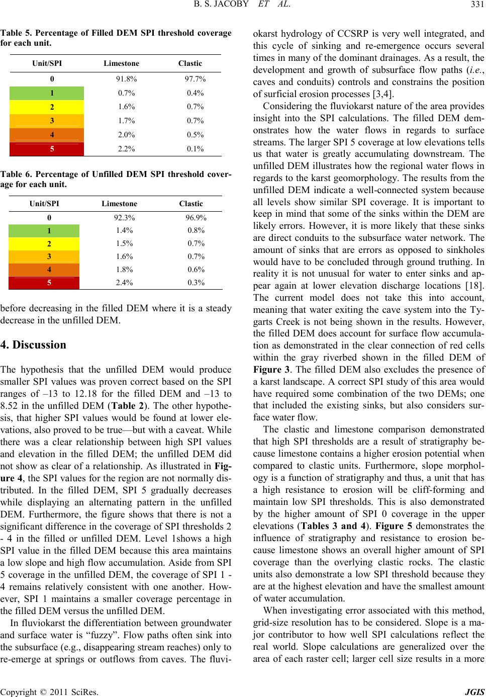
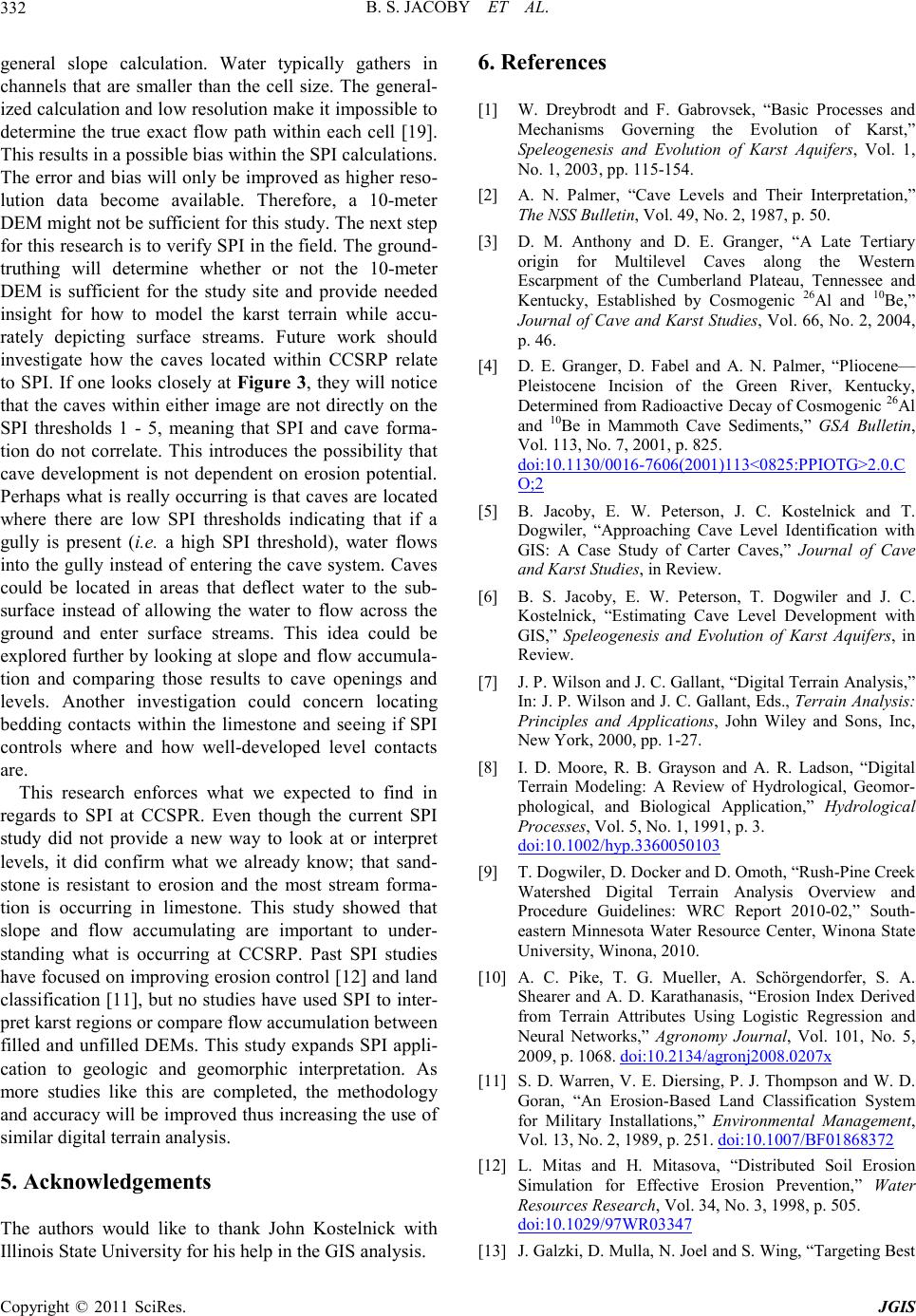
Journal of Geographic Information System, 2011, 3, 323-333
doi:10.4236/jgis.2011.34030 Published Online October 2011 (http://www.SciRP.org/journal/jgis)
Identifying the Stream Erosion Potential of Cave Levels in
Carter Cave St ate Resort Park, Kentuck y, USA
Brianne Spence Jacoby1, Er ic W a d e Pe t erson1, Toby Dogwiler2
1Department of Geology Geography, Illinois State University, Normal, USA
2Department of Geosciences, Winona State University, Winona, USA
Received July 8, 2011; revised August 16, 2011; accepted August 25, 2011
Abstract
Cave levels, passages found at similar elevations and formed during the same constant stream base level
event, reveal information about paleoclimates and karst geomorphology. The investigation presented here
examines how Stream Power Index (SPI) relates to cave levels. The study area, Carter Caves State Resort
Park (CCSRP), is a fluviokarst system in northeastern Kentucky containing multiple cave levels. SPI deter-
mines the erosive power overland flow based on the assumption that flow accumulation and slope are pro-
portional to potential for sediment entrainment. Part of this digital terrain analysis requires the creation of a
flow accumulation raster from a digital elevation model (DEM). In creating the flow accumulation raster,
one has the option to fill depressions (also considered errors) within the DEM. Filling these depressions, or
“sinks,” creates a well-connected stream network; however it also removes possible sinkholes from the DEM.
This paper also investigates the effects a filled and an unfilled DEM have on SPI and what each reveals
about erosion potential in the area. The data shows that low elevations within the filled DEM maintain a high
SPI value when compared to the unfilled DEM. The filled DEM also created a stream network similar to re-
ality. The unfilled DEM demonstrated similar SPI results between all levels, indicating a well-connected
karst system. In order to truly understand the mechanics of this system, a combination of these two DEMs is
required.
Keywords: Karst, Erosion, Geomorphology, Speleogenesis, Terrain Analysis
1. Introduction
The term karst describes terrain that contains both surfi-
cial and subterranean landforms that form through dis-
solution. Dissolution occurs when water, rich in carbon
dioxide, dissolves the calcite in limestone or other cal-
cium-bearing rocks and removes it through the aqueous
solution [1]. The landforms produced through this proc-
ess include, but are not limited to, sinkholes, cave cav-
erns, sinking streams, and passageways. Dissolution cre-
ates a system with waterways flowing in both vertical
and horizontal directions. Passage development is de-
pendent on a variety of factors, including base flow ele-
vation of the streams, stratigraphy, the movement of wa-
ter in the unsaturated zone to underlying bedrock,
chemical variations, and variations in discharge [2]. Ac-
tive dissolution and extended periods of constant base
level, allow for large passages to develop at or near the
current base level elevation. When the regional base
level lowers, river incision rates increase and groundwa-
ter flow is deflected to lower elevations [3]. Dissolution
in passages that were abandoned by groundwater flow is
limited or stopped as a result of this regional hydrologic
change.
Cave levels are identified as a group of passages found
at similar elevations. It is understood that these passages
are created at the same time when the region’s surface
waters maintained a static base elevation. Consequently,
cave levels are significant landforms left in the rock re-
cord that can help in deciphering the timing of cave sys-
tem development. Multile vel cave systems contain a his-
tory of episodic lowering of the local base level in re-
sponse to regional discharge changes. Deciphering where
the flow has changed from predominantly horizontal
flow to vertical flow is considered to be the level bound-
ary [2]. Cave levels have been used to develop speleo-
genic histories of Mammoth Cave [4], the Cumberland
Plateau region [3], and the Carter Caves karst area [5,6].

B. S. JACOBY ET AL. 324
Additional i nsight on the evol ution of karst syste ms pro-
vide greater understanding of the systems’ complicated
mechanics and are important to understanding the pa-
leoenvironment.
Digital terrain analysis (DTA) is a quantitative
GIS-based technique for analyzing topography and geo-
morphic processes at a variety of scales using digital
elevation models (DEMs) [7]. The growth in availability
of accurate high-resolution DEMs collected using Li-
DAR has opened up opportunities to understand and pre-
dict landscape processes related to erosion, contaminant
transport, and other related phenomena. Furthermore,
DTA has become a tool for studying topographically-
related landscape features such as soils, vegetation, and
even wildlife.
DTA is based on the derivation and analysis of primary
and secondary topographic attributes. Primary terrain at-
tributes include topographic characteristics such as aspect,
slope, catchment area, and profile curvature which are
directly measurable from a DEM or topographic map.
Secondary topographic attributes are derived by combin-
ing primary attributes mathematically. Generally, secon-
dary attributes are indices that predict and describe the
spatial variability of hydrological, geomorphological, and
biological processes across the landscape [8]. Topographic
attribute values are typically calculated (e.g., with Raster
Calculator in ArcGIS) for each cell in the DEM raster.
Thus, the accuracy and precision of the attribute derivation
and their predictive power are directly related to the reso-
lution of the DEM.
The Stream Power Index (SPI) is a secondary topog-
raphic attribute derived from slope and the contributing
area of flow accumulation. Despite its name, the SPI
evaluates erosive power across the whole landscape, not
just in streams. By highlighting areas with large catch-
ments and steep slopes the SPI predicts contributing ar-
eas where the erosive power of overland flow will be the
highest [7]. In the absence of regional discharge data,
SPI can also serve as a simple to employ surrogate for
identifying areas at risk for intense stream erosion, espe-
cially in relation to high-magnitude precipitation events.
Use of the SPI, as with all DTA, necessarily involves
field-based verification to determine the threshold SPI
values that serve as a minimum for making useful pre-
dictions about erosive potential across the landscape [9].
SPI can also be used to locate and identify the erosion
potential of ephemeral gullies. Ephemeral gullies are
typically observed after high-magnitude, low frequency
precipitation events that trigger overland flow. In karst
areas, such overland flow occurs when subsurface flow
paths become inundated and excess flow is forced to
follow surface flow routes. Such gullies typically “heal”
between overland flows events through mass wasting
processes such as creep and hill slope slump. However,
subsequent flow events will often lead to re-initiation of
gullying processes along the same locations. Pike et al.
[10] used various terrain analyses, including SPI, to
model erosion potential of ephemeral gullies and then
compared those results to real-world conditions. They
found that about 80% of the calculated SPI values, which
were above the critical predictive threshold, successfully
identified areas of observed gully formation.
Other studies that have used SPI, focus on general
topics such as erosion, sediment transport, and geomor-
phology [8] and more specific purposes such as land
classification for the military [11]. Mitas and Mitasova
[12] used SPI to find areas that were at risk for erosion in
order to improve erosion prevention practices. They
found that variations within a terrain determine how ero-
sion patterns will evolve over a landscape. In addition to
terrain, they discussed that land cover will influence how
water flow paths form.
Galzki et al. [13] used LiDAR data to identify SPI
within two portions of the Minnesota River Basin; one
watershed was approximately 100 square kilometers
while the other was 20 square kilometers. The data were
provided at a 1-meter scale, but the authors resampled
the data to 3-meters in order to reduce processing time
while maintaining high accuracy. The majority of the
study area was of low to moderate relief. Terrain attrib-
utes are more straightforward in regions with high relief
because flow routes are easier to distinguish. Therefore,
more caution is required when interpreting terrain as an
area’s relief decreases. The authors found the previous
statement to be true and concluded that the SPI predic-
tions in areas with extremely low relief were likely unre-
alistic. With the results of this study, researchers identi-
fied areas that were at risk of erosion. When they
ground-truthed those results, they found that out of the
15 areas visited, 14 were identified as being at risk of
erosion. Seven (7) of those 14 areas contained gullies.
Galzki et al. successfully identified features that could be
contributing networks for transporting contaminants
from agricultural fields. The results of this study are be-
ing used to bring forth water quality and conservation
efforts to the area.
Carter Caves State Resort Park (CCSRP) is located in
Carter County. The park consists of approximately 106
square kilometers of deeply incised valleys, characteris-
tic of the Cumberland Plateau [14]. The elevation range
in this area is between approximately 197 meters and 345
meters above sea level, with the maximum land slope
being 41˚ in the bottom of the river valleys. The Borden
Formation is the oldest formation in the park, consisting
of fine-grained sandstone, siltstone, and shale. The Bor-
den Formation is considered to control the tributary

B. S. JACOBY ET AL. 325
down cutting in the area [15]. This unit is overlain by the
Newman Limestone, which contains the caves the area is
known for. The Newman Limestone contains the Upper
Renfro Formation, the St. Louis Limestone, the St.
Genevieve Limestone, and the Upper Newman Forma-
tion. These limestone formations vary in color, grain
sorting, and stratigraphic structures. Capping the New-
man is the Pennington Formation, which includes the
Carter Caves and Lee sandstones. The Pennington For-
mation is the park’s cliff-forming unit.
In a previous work, Jacoby et al. [5,6] used GIS, a
cave database for CCSPR, and a 10-meter DEM to iden-
tify levels within CCSRP. The authors found two differ-
ent options for the amount of levels within the park. Op-
tion 1 consists of four levels and Option 2 consists of
five levels. Levels 1 - 3 cover the same extent for both
options but Level 4, Option 1 is split into levels 4 and 5
in Option 2. Distinguishing between four a nd five levels
is important when learning about the region’s speleo-
genesis. This st udy will use the results of Jacob y et al. [5]
for the location and elevations of existing cave levels.
The project presented here is designed to take SPI ap-
plication a step further. Currently, SPI research focuses
on areas in erosion prevention and land classification.
Here SPI is used to determine if the erosion patterns
within a karst system correlate with cave levels. SPI will
be applied to CCSRP in northeastern Kentucky in order
to compare how erosion potential values compare to cave
levels within CCSRP (Figure 1). Note that in creating a
SPI dataset, one must create a stream network. This
process requires a decision to be made on whether or not
to fill “sinks” within the DEM. Filling sinks is a practice
that removes depressions, or possible errors, within the
dataset. These depressions collect water and eliminate
flow from continuing downstream (Figure 2). However
by filling sinks, one is assuming that all depressions are
error s. Arnold [16] suggest s that the size of these dep ress-
sions should be considered before they are filled. Based
Figure 1. Location of CCSRP. Note that gray-scale image shown is only a portion of the DEM used in this study.

B. S. JACOBY ET AL. 326
Figure 2. Schematic of how filling the DEM tool works. a) A
DEM without sinks filled. Water enters the sink, but does
not leave. b) A DEM with the sinks filled. Water runs over
the sink and conti nues d ownstream.
on the fact that the study area is karst terrain and depres-
sions are likely, it would be acceptable to not fill the
sinks within the DEM. However by not filling the sinks,
a well-connected stream network will not be created. A
poorly connected stream network will result in less water
accumulation downstream, and therefore, some gullies
will demonstrate a smaller erosion potential than reality.
In order to gain a complete understanding of how filling
sinks within the CCSRP DEM will effect prediction of
the region’s erosion potential, there will be t wo different
SPI datasets created; one representing erosion potential
of a filled DEM and the other representing the erosion
potential of an unfilled DEM. One hypothesis is that
there are a smaller amount of SPI values in the unfilled
DEM versus the filled DEM. This is based on the as-
sumption that there will be less flow accumulation cells
in the unfilled DEM. Another hypothesis is that there are
higher SPI values in cave levels at lower elevations.
Streams at lower elevations tend to be larger and have a
greater amount of water moving through them at one
time as compared to streams at higher elevations. This is
because lower elevation streams have a larger contribut-
ing area for water.
2. Materials and Methods
The procedures outlined by Galzki et al. [13] and Dog-
wiler et al. [9] were followed for this project. A Geo-
graphic Information System (GIS) was used to perform
the analysis along with the cave level elevations found
by Jacoby et al. [5] and a 10-meter DEM that was down-
loaded from seamless.usgs.gov. According to the Na-
tional Standard for Spatial Data Accuracy (NSSDA)
horizontal accuracy associated with these 10 meter
DEMs is approximately ±13.906 meters while the verti-
cal accuracy is approximately ±0.3632 meters [17]. This
DEM covers an area that is approximately 73 square
kilometers. The resolution of the DEM is important to
consider in respect to the size of the study area. If look-
ing at a small landscape feature such as a pasture or
small farm, a high resolution DEM is required [9].
However if looking at a larger area, such as a county or
state park, high resolution DEMs can provide too much
detail for the area in question. It is also important to note
that not all areas have high resolution DEMs or LiDAR
data available. The smallest DEM resolution available
for this area is 10 meters and that is why a higher resolu-
tion option was not explored.
The first step taken in this study was to create a raster
that represented the elevation range of each cave level
found by Jacoby et al. [5]. Six (6) rasters were created in
total (Table 1): Level 1 (L1) ranging from 214 - 228
meters, Level 2 (L2) ranging from 228 - 240 meters,
Level 3 (L3) ranging from 240 - 253 meters, Level
4-Option 1 (L4-Op1) ranging from 253 - 274 meters,
Level 4-Option 2 (L4-Op2) ranging from 253 - 263 me-
ters and Level 5-Option 2 (L5-Op2) ranging from 236 -
274 meters. The rasters were created using Equation (1):
Level i = [CCSRP_DEM] > lower_range &
[CCSRP_DEM] <= upper_range (1)
where Level i refers to the level (and option) of interest,
CCSRP_DEM is the 10-meter DEM used for this study,
lower_range is the lo wer elevation of the given level, and
upper_range is the upper elevation of the given level
(Table 1). Another raster calculation was performed to
identify the area of clastic rocks overlying the limestone
units. This raster included all cells that were greater than
274 meters, which is the contact elevation between the
limestone and clastic units [5]. An equation similar to (1)
was used, with only one reference to [CCSRP_DEM]
and identified cells greater than 274 meters.
A filled DEM was then created using the “fill” tool in
Table 1. Level Elevation Ranges modified from Jacoby et al.
[5].
Level Ele vation Range (m)
L5-Op2 263 - 274
L4-Op2 253 - 263
L4-Op1 253 - 274
L3 240 - 253
L2 228 - 240
L1 214 - 228
(a)
(b)

B. S. JACOBY ET AL. 327
ArcMap 9.3.1, which finds depressions within the DEM
and fills those that inhibit flow downhill in order to cre-
ate a realistic stream network. Next, SPI calculations for
both a filled and unfilled DEM were performed using
Equation ( 2).
SPI = (flow accumulation)*(slope) (2)
Flow accumulation (or upslope contributing area)
summarizes the amounts of cells that flow into a single
cell whereas slope represents the maximum rate of
change between a cell and its neighbors. The flow accu-
mulation raster was derived using Hydrology tools avai-
lable in ESRI’s ArcMap™ 9.3.1. The surface analyst
tools in ArcMap™ 9.3.1 were used to derive a slope
raster. All rasters were manipulated as directed by Dog-
wiler et al. [9] until a Raw SPI raster was determined.
Statistical analyses were performed to calculate the
percentiles (1st - 99th) of the SPI data. The percentile
value s were b rought b ack in to the GI S to de termine fi nal
SPI thresholds. The percentile range used to choose a
threshold typically depends on the regional geology and
geomorphology as well as the purpose of the research [9].
Researchers working in flat landscapes typically choose
lower percentiles than those working in steep landscapes.
The thresholds for this site were based on past experi-
ences with SPI thresholds and knowledge of CCSRP.
The thresholds presented here are a conservative guess,
but they reproduce artificial stream networks created by
Jacoby et al. [5]. Five thresholds were chosen with val-
ues ranging between the 99th, 98th, 97th, 96th and 95th
percentiles. These values were given a threshold value of
5 through 1 respectfully, with 5 having the greatest ero-
sion potential. A sixth threshold, value of 0, was given to
the remaining percentile values (Table 2). Note that the
Raw SPI values shown below vary between the filled and
unfilled DEMs. This is because the unfilled DEM had a
smaller accumulation raster. Although there was this
difference, the SPI thresholds are the same. Unfilled Raw
SPI values of 4.38 - 8.52 represent the highest erosion
potential for its DEM and are given a SPI threshold of 5.
A larger flow accumulation raster resulted in higher Raw
SPI values for the filled DEM. Raw SPI values of 5.41 -
12.18 represent the highest erosion potential for its DEM
and are also given a SPI threshold of 5. The SPI thresh-
olds represent the erosion risk of those cells for each
DEM, regardless of how the original SPI values compare
between the DEMs.
Using Equation (3), raster calculations were performed
to see how many of the grid cells within each level con-
tained the various SPI thresholds.
true Level i cells & [CCSRP_SPI] > lower_value &
[CCSRP_SPI] <= upper_value (3)
where true Level i refers to the level cells of interest and
CCSRP_SPI refers to the SPI raster, lower_value is the
lower Raw SPI value of the SPI threshold in question,
and upper_value is the upper Raw SPI value of the SPI
threshold in question (Table 2) . Seventy-two (7 2) calcu-
lations were performed in total (36 calculations per
DEM).
Next, the cells within the clastic raster that contained
each of the SPI thresholds were counted. Twelve (12)
calculations were performed in total (6 per DEM). Equa-
tion (3) was used. Note that the variables ranged based
on the clastic raster and the SPI threshold in question.
The final step was to calculate the percentage of cover-
age of each SPI threshold within each level or clastic
raster. Equation (4) was used:
% SPI threshold coverage = [(SPI threshold cells within
Level i)/(total cells within Level i)]*100 (4)
where SPI threshold corresponds to the SPI threshold in
question and Le vel i refers to the level of interest.
3. Results
Generation of a stream network using SPI values creates a
continuous network in the filled DEM (Figure 3(a)) and
an irregular network in the unfiled DEM (Figure 3 (b)).
These patterns are the result of different flow accumula-
tion rasters, the filled DEM having a larger one com-
Table 2. This table outlines SPI thresholds used for this study. Note that the Raw SPI values are higher in the filled Dem than
the unfilled DEM.
SPI Threshold Percentile Filled Raw SPI Value Unfilled Raw SPI Value
0 1st - 94th –13.82 - 2.87 –13.82 - 2.49
1 95th 2.87 - 3.06 2.49 - 2.78
2 96th 3.06 - 3.54 2.78 - 3.14
3 97th 3.54 - 4.23 3.14 - 3.62
4 98th 4.23 - 5.41 3.62 - 4.38
5 99th 5.41 - 12.18 4.38 - 8.52

B. S. JACOBY ET AL. 328
(b)
(a)
(c) (d)
Figure 3. Visual of SPI designation using a) a filled DEM and b) an unfilled DEM. Figures c) and d) show a large scale depic-
tion of Horn Hollow (outlined area). SP I 0 is not shown because it equates to ev ery cell but those alrea dy classified as SPI. If
it w as shown, the other de tail w ould be l ost. Al so note th at all area depicte d as “L EVELS” is also l imesto ne. The st ream net-
work in the unfilled DEM is discontinuous compared to the filled DEM.

B. S. JACOBY ET AL. 329
pared to the unfilled DEM. In the filled DEM, SPI 5 is
primarily found within existing waterways. SPI 5 in the
unfilled DEM is also found in existing waterways, except
the cells do not extend the full distance of the actual
channel.
The difference in coverage between the filled and un-
filled DEMs is evident in lower elevations of Figure 3
(closest to the riverbed). The coverage of SPI 5 in the
filled DEM is greater than the unfilled DEM whereas SPI
1 has a higher coverage in the unfilled DEM than the
filled DEM. Approximately 10% of the area is desig-
nated with SPI values above the 95% threshold (Tables 3
and 4). Using the Filled DEM generates a SPI coverage
that illustrates more variability than the unfilled DEM
(Figure 4). However, the coverage percentages for each
threshold group are rather stable among the levels. The
percentages listed indicate how much of the entire level
is covered by a given percentile. For example in the
filled DEM, raster cell values between 5.41 and 12.18
make up the 99th percentile. Out of all the cells that con-
stitute Level 1, 5% of those are in the 99th percentile of
SPI values. The coverage of SPI 5 appears to increase as
level elevation decreases in the filled DEM, indicating
the highest erosion potential is at the lowest elevations.
The other threshold values, 1 - 4 appear to stay consis-
tently between the 0.5% and 2.5%. The percentage of
area designated as SPI 0 decreases as level elevation de-
creases, indicating that there is smaller erosion potential
at higher elevations.
The SPI coverage in the unfilled DEM does not show
the same pattern as the filled DEM. The coverage of SPI
5 does decrease with elevation, but Level 2 maintains the
highest percentage of coverage. Note that the percentage
of coverage is overall higher in SPI 5 values within the
filled DEM verses the unfilled DEM. SPI 1 - 4 values in
Level 1 maintain a higher coverage percentage in the
unfilled DEM than the filled DEM. Level 2 appears to
have similar coverage in the filled and unfilled DEM.
Level 3 has lower coverage of SPI 1 - 4 values in the
unfilled DEM than the filled DEM. The coverage of SPI
1 - 4 in Level 4, Option 1, Level 4, Option 2, and Level 5,
Option 2 appear to be similar in both DEMs.
Table 5 shows the coverage of SPI across the lime-
stone and clastic units in the filled DEM while Table 6
shows the coverage of SPI across the limestone and clas-
tic units in the unfilled DEM. Figure 5 provides a visual
Table 3. Percentage of Filled DEM SPI threshold coverage for each level.
–13 - 28.87 2.7 - 3.06 3.06 - 3.54 3.54 - 4.23 4.32 - 5.41 5.41 - 12.18
Level/SPI 0 1 2 3 4 5
1 88.42% 0.9% 2.1% 1.9% 1.7% 5.0%
2 89.5% 1.1% 1.7% 1.7% 2.3% 3.7%
3 92.5% 0.6% 1.4% 1.4% 1.8% 2.3%
4, option 1 92.6% 0.7% 1.5% 1.7% 2.1% 1.4%
4, option 2 91.9% 0.7% 1.6% 1.7% 2.2% 2.0%
5, option 2 93.0% 0.7% 1.5% 1.8% 2.0% 1.0%
Table 4. Percentage of Unfilled DEM SPI threshold coverage for each level.
–13 - 28.87 2.7 - 3.06 3.06 - 3.54 3.54 - 4.23 4.32 - 5.41 5.41 - 12.18
Level/SPI 0 1 2 3 4 5
1 88.7% 2.0% 2.0% 2.2% 2.0% 3.1%
2 89.0% 2.0% 2.1% 1.8% 1.9% 3.3%
3 92.0% 1.3% 1.3% 1.4% 1.6% 2.5%
4, option 1 91.2% 1.3% 1.4% 1.6% 1.8% 2.0%
4, option 2 91.2% 1.3% 1.4% 1.7% 1.9% 2.5%
5, option 2 92.4% 1.2% 1.3% 1.6% 1.8% 1.7%

B. S. JACOBY ET AL. 330
Figure 4. Graph depicting relationship between filled (a) and unfilled (b) DEMs’ SPI threshold and Level. Note that Level 1 is
at the lowest elevation and Level 4, Option 1 and Level 5, Option 2 are the highest in elevation.
Figure 5. Graph depicting relationship between filled and unfilled DEMs’ SPI threshold and the percentage of coverage.
depiction of those results. Notice how in both DEMs, the
percentage of coverage increases with SPI threshold
within the limestone but decreases within the sandstone.
This indicates that the limestone has a higher erosion
potential. The main difference between the two DEMs is
that erosion potential of the clastic rock increases slightly
(a) (b)

B. S. JACOBY ET AL.331
Table 5. Percentage of Filled DEM SPI threshold coverage
for each unit .
Unit/SPI Limestone Clastic
0 91.8% 97.7%
1 0.7% 0.4%
2 1.6% 0.7%
3 1.7% 0.7%
4 2.0% 0.5%
5 2.2% 0.1%
Table 6. Percentage of Unfilled DEM SPI threshold cover-
age for each unit.
Unit/SPI Limestone Clastic
0 92.3% 96.9%
1 1.4% 0.8%
2 1.5% 0.7%
3 1.6% 0.7%
4 1.8% 0.6%
5 2.4% 0.3%
before decreasing in the filled DEM where it is a steady
decrease in the unfilled DEM.
4. Discussion
The hypothesis that the unfilled DEM would produce
smaller SPI values was proven correct based on the SPI
ranges of –13 to 12.18 for the filled DEM and –13 to
8.52 in the unfilled DEM (Table 2). The other hypothe-
sis, that higher SPI values would be found at lower ele-
vations, also proved to be true—but with a caveat. While
there was a clear relationship between high SPI values
and elevation in the filled DEM; the unfilled DEM did
not show as clear of a relationship. As illustrated in Fig-
ure 4, the SPI values for the region are not normally dis-
tributed. In the filled DEM, SPI 5 gradually decreases
while displaying an alternating pattern in the unfilled
DEM. Furthermore, the figure shows that there is not a
significant difference in the coverage of SPI thresholds 2
- 4 in the filled or unfilled DEM. Level 1shows a high
SPI value in the filled DEM because this area maintains
a low slope and high flow accumulation. Aside from SPI
5 coverage in the unfilled DEM, the coverage of SPI 1 -
4 remains relatively consistent with one another. How-
ever, SPI 1 maintains a smaller coverage percentage in
the filled DEM versus the unfilled DEM.
In fluviokarst the differentiation between groundwater
and surface water is “fuzzy”. Flow paths often sink into
the subsurface (e.g., disappearing stream reaches) only to
re-emerge at springs or outflows from caves. The fluvi-
okarst hydrology of CCSRP is very well integrated, and
this cycle of sinking and re-emergence occurs several
times in many of the dominant dr ainages. As a result, the
development and growth of subsurface flow paths (i.e.,
caves and conduits) controls and constrains the position
of surficial erosion processes [3,4].
Considering the fluviokarst nature of the area provides
insight into the SPI calculations. The filled DEM dem-
onstrates how the water flows in regards to surface
streams. The larger SPI 5 coverage at low elevations tells
us that water is greatly accumulating downstream. The
unfilled DEM illustrates how the regional water flows in
regards to the karst geomorphology. The results from the
unfilled DEM indicate a well-connected system because
all levels show similar SPI coverage. It is important to
keep in mind that some of the sinks within the DEM are
likely errors. However, it is more likely that these sinks
are direct conduits to the subsurface water network. The
amount of sinks that are errors as opposed to sinkholes
would have to be concluded through ground truthing. In
reality it is not unusual for water to enter sinks and ap-
pear again at lower elevation discharge locations [18].
The current model does not take this into account,
meaning that water exiting the cave system into the Ty-
garts Creek is not being shown in the results. However,
the filled DEM does account for surface flow accumula-
tion as demonstrated in the clear connection of red cells
within the gray riverbed shown in the filled DEM of
Figure 3. The filled DEM also excludes the presence of
a karst landscape. A correct SPI study of this area would
have required some combination of the two DEMs; one
that included the existing sinks, but also considers sur-
face water flow.
The clastic and limestone comparison demonstrated
that high SPI thresholds are a result of stratigraphy be-
cause limestone contains a higher erosion potential when
compared to clastic units. Furthermore, slope morphol-
ogy is a func tion of strati graphy and thus, a unit t hat has
a high resistance to erosion will be cliff-forming and
maintain low SPI thresholds. This is also demonstrated
by the higher amount of SPI 0 coverage in the upper
elevations (Tables 3 and 4). Figure 5 demonstrates the
influence of stratigraphy and resistance to erosion be-
cause limestone shows an overall higher amount of SPI
coverage than the overlying clastic rocks. The clastic
units also demonstrate a low SPI threshold because they
are at the highest elevation and have the smallest amount
of water accumulation.
When investigating error associated with this method,
grid-size resolution has to be considered. Slope is a ma-
jor contributor to how well SPI calculations reflect the
real world. Slope calculations are generalized over the
area of each raster cell; larger cell size results in a more

B. S. JACOBY ET AL. 332
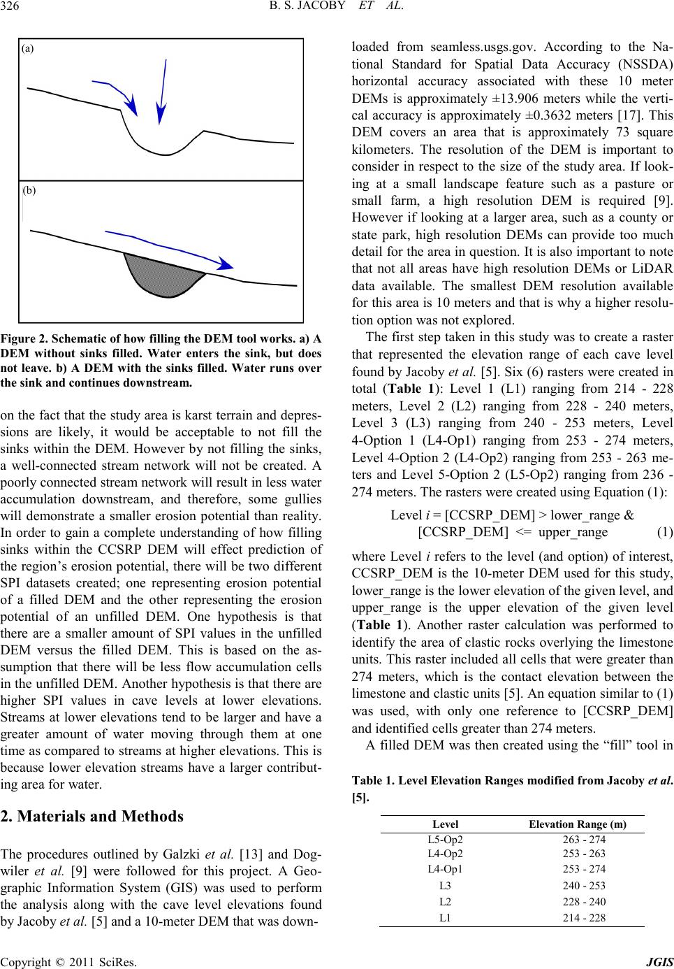
general slope calculation. Water typically gathers in
channels that are smaller than the cell size. The general-
ized calculation and lo w resolution make it i mpossible to
determine the true exact flow path within each cell [19].
This results in a possible bias within the SPI calculations.
The error and bias will only be improved as higher reso-
lution data become available. Therefore, a 10-meter
DEM might not be sufficient for this study. The next step
for this research is to verify SPI in the field. The ground-
truthing will determine whether or not the 10-meter
DEM is sufficient for the study site and provide needed
insight for how to model the karst terrain while accu-
rately depicting surface streams. Future work should
investigate how the caves located within CCSRP relate
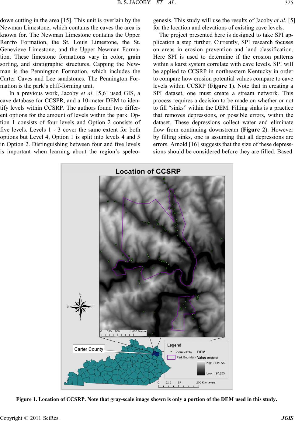
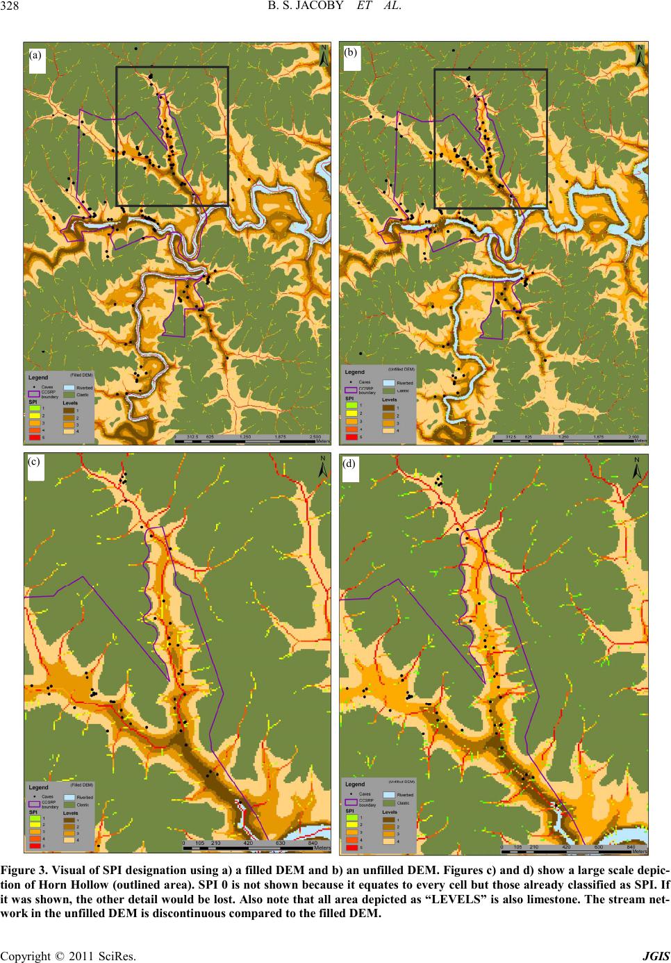
to SPI. If one looks closely at Figure 3, they will notice
that the caves within either image are not directly on the
SPI thresholds 1 - 5, meaning that SPI and cave forma-
tion do not correlate. This introduces the possibility that
cave development is not dependent on erosion potential.
Perhaps what is really occurring is that caves are located
where there are low SPI thresholds indicating that if a
gully is present (i.e. a high SPI threshold), water flows
into t he gull y instead of ente ring the cave sys tem. Ca ves
could be located in areas that deflect water to the sub-
surface instead of allowing the water to flow across the
ground and enter surface streams. This idea could be
explored further by looking at slope and flow accumula -
tion and comparing those results to cave openings and
levels. Another investigation could concern locating
bedding contacts within the limestone and seeing if SPI
controls where and how well-developed level contacts
are.
This research enforces what we expected to find in
regards to SPI at CCSPR. Even though the current SPI
study did not provide a new way to look at or interpret
levels, it did confirm what we already know; that sand-
stone is resistant to erosion and the most stream forma-
tion is occurring in limestone. This study showed that
slope and flow accumulating are important to under-
standing what is occurring at CCSRP. Past SPI studies
have focused on improving erosion control [12] and land
classification [11], but no studies have used SPI to inter-
pret karst regions or compare flow accumulation between
filled and unfilled DEMs. This study expands SPI appli-
cation to geologic and geomorphic interpretation. As
more studies like this are completed, the methodology
and accuracy will be improved thus increasing the use of
similar digital terrain analysis.
5. Acknowledgements
The authors would like to thank John Kostelnick with
Illinois State University for his help in the GIS analysis.
6. References
[1] W. Dreybrodt and F. Gabrovsek, “Basic Processes and
Mechanisms Governing the Evolution of Karst,”
Speleogenesis and Evolution of Karst Aquifers, Vol. 1,
No. 1, 2003, pp. 115-154.
[2] A. N. Palmer, “Cave Levels and Their Interpretation,”
The NSS Bulletin, Vol. 49, No. 2, 19 8 7, p. 5 0 .
[3] D. M. Anthony and D. E. Granger, “A Late Tertiary
origin for Multilevel Caves along the Western
Escarpment of the Cumberland Plateau, Tennessee and
Kentucky, Established by Cosmogenic 26Al and 10Be,”
Journal of Cave and Karst Studies, Vol. 66, No. 2, 2004,
p. 46.
[4] D. E. Granger, D. Fabel and A. N. Palmer, “Pliocene—
Pleistocene Incision of the Green River, Kentucky,
Determined from Radioactive Decay of Cos mogenic 26Al
and 10Be in Mammoth Cave Sediments,” GSA Bulletin,
Vol. 113, No. 7, 2001, p. 825.
doi:10.1130/0016-7606(2001)113<0825:PPIOTG>2.0.C
O;2
[5] B. Jacoby, E. W. Peterson, J. C. Kostelnick and T.
Dogwiler, “Approaching Cave Level Identification with
GIS: A Case Study of Carter Caves,” Journal of Cave
and Karst Studies, in Review.
[6] B. S. Jacoby, E. W. Peterson, T. Dogwiler and J. C.
Kostelnick, “Estimating Cave Level Development with
GIS,” Speleogenesis and Evolution of Karst Aquifers, in
Review.
[7] J. P. Wilson and J. C. Gallant, “Digital Terrain Analysis,”
In: J. P. Wilson and J. C. Gallant, Eds., Terrain Analysis:
Principles and Applications, John Wiley and Sons, Inc,
New York, 2000, pp. 1-27.
[8] I. D. Moore, R. B. Grayson and A. R. Ladson, “Digital
Terrain Modeling: A Review of Hydrological, Geomor-
phological, and Biological Application,” Hydrological
Processes, Vol. 5, No. 1, 1991, p. 3.
do i:10.1002/hyp.3360050103
[9] T. Dogwiler, D. Docker and D. Omoth, “Rush-Pine Creek
Watershed Digital Terrain Analysis Overview and
Procedure Guidelines: WRC Report 2010-02,” South-
eastern Minnesota Water Resource Center, Winona State
University, Winona, 2010.
[10] A. C. Pike, T. G. Mueller, A. Schörgendorfer, S. A.
Shearer and A. D. Karathanasis, “Erosion Index Derived
from Terrain Attributes Using Logistic Regression and
Neural Networks,” Agronomy Journal, Vol. 101, No. 5,
2009, p. 10 68. doi:10.2134/agronj2008.0207x
[11] S. D. Warren, V. E. Diersing, P. J. Thompson and W. D.
Goran, “An Erosion-Based Land Classification System
for Military Installations,” Environmental Management,
Vol. 13, No. 2, 1989, p. 251. doi:10.1007/BF01868372
[12] L. Mitas and H. Mitasova, “Distributed Soil Erosion
Simulation for Effective Erosion Prevention,” Water
Resources Research, Vol. 34, No. 3, 1998, p. 505.
doi:10.1029/97WR03347
[13] J. Galzki, D. Mulla, N. Joel and S. Wing, “Targeting Best

B. S. JACOBY ET AL. 333
Management Practices (BMPs) to Critical Portions of the
Landscape: Using Selected Terrain Analysis Attribu tes to
Identify High-Contributing Areas Relative to Nonpoint
Source Pollution,” Minnesota Department of Agriculture,
2008.
[14] A. S. Engel and S. A. En gel, “A Field Guid e for the Karst
of Carter Caves State Resort Park and the Surrounding
Area, Northeastern Kentucky,” In: A. S. Engel, Ed., Field
Guide to Cave and Karst Lands of the United States,
Karst Waters Institute Special Publication 15, Karst
Waters Institute, Leesburg, 2009, pp. 154-171.
[15] G. D. Ochsenbein, “Origin of Caves in Carter Caves State
Park, Carter County, Kentucky,” Bowling Green State
University, Bowling Green, 1974.
[16] N. Arnold, “A New Approach for Dealing with Depre-
ssions in Digital Elevation Models When Calculating Flo w
Accumulation Values,” Progress in Physical Geo-
graphy, Vol. 34, No. 6, 2010, p. 781.
doi:10.1177/0309133310384542
[17] T. Blak , “DEM Quality Assessment,” In: D. F. Ma une, Ed.,
Digital Elevation Model Technologies and Applications:
The DEM Users Manual, American Society for Photo-
grammetry and Remote Sensing, Bethesda, 2007, pp. 425-
448.
[18] C. G. Groves and A. D. Howard, “Early Development of
Karst Systems; 1, Preferential Flow Path Enlargement
under Laminar Flow,” Water Resources Research, Vol.
30, No. 10, 1 99 4, p. 2837. doi:10.1029/94WR01303
[19] J. C. Gallant, M. F. Hutchinson and J. P. Wilson, “Future
Directions for Terrain Analysis,” In: J. P. Wilson and J. C.
Gallant, Eds., Terrain Analysis: Principles and Appli-
cations, John Wiley and Sons, Inc, New York, 2000, pp.
423-427.