Journal of Geographic Information System, 2011, 3, 279-289
doi:10.4236/jgis.2011.34024 Published Online October 2011 (http://www.SciRP.org/journal/jgis)
Hydrologic Modeling of the Bouregreg Wate rshed
(Morocco) Using GIS and SWAT Model
Abdelh am id Fadil1, Hassan Rhina n e 1, Abdelhadi Kaoukaya1,
Youne s s Kh a rchaf1, Omar Ala mi Bachir2
1Geosciences Laboratory, Faculty of Sciences-Ain Chock, Hassan II Univertsity, Casablanca, Morocco
2Hassania School of Public Works, Casablanca, Morocco
Received August 6, 2011; revised September 10, 2011; accepted September 22, 2011
Abstract
The study of water resources at watershed scale is widely adopted as approach to manage, assess and simu-
late these important natural resources. The development of remote sensing and GIS techniques has allowed
the use of spatially and physically based hydrologic models to simulate as simply and realistically as possible
the functioning of watershed systems. Indeed, the major constraint that has hindered the expansion use of
these tools was the unavailability or scarcity of data especially in the developing countries. In this context,
the objective of this study is to model the hydrology in the Bouregreg basin, located at the north-central of
Morocco, using the Soil and Water Assessment Tool (SWAT) in order to understand and determine the dif-
ferent watershed hydrological processes. Thus, it aims to simulate the stream flow, establish the water bal-
ance and estimate the monthly volume inflow to SMBA dam situated at the basin outlet. The ArcSWAT in-
terface implemented in the ArcGIS software was used to delineate the basin and its sub-components, com-
bine the data layers and edit the model database. The model parameters were analyzed, ranked and adjusted
for hydrologic modeling purposes using daily temporal data series. They were calibrated using an
auto-calibration method based on a Shuffled Complex Evolution Algorithm from 1989 to 1997 and validated
from 1998 to 2005. Based on statistical indicators, the evaluation indicates that SWAT model had a good
performance for both calibration and validation periods in Bouregreg Watershed. In fact, the model showed a
good correlation between the observed and simulated monthly average river discharge with R² and Nash co-
efficient of about 0.8. The water balance components were correctly estimated and the SMBA dam inflow
was successfully reproduced with R² of 0.9. These results revealed that if properly calibrated, SWAT model
can be used efficiently in semi-arid regions to support water management policies.
Keywords: Hydrologic Modeling, Water Balance, Calibration, Bouregreg Watershed, GIS, SWAT, Arcswat
1. Introduction
The water is the most important natural resource espe-
cially in the arid or semi-arid zones that face high popu-
lation growth, scarcity of freshwater, irregularity of rain-
fall, excessive land use change and increasing vulner-
ability to risks s uch of dro ught, desertificatio n and pollu-
tion. Thus, the availability and the sustainable use of this
resource become the core of the local and national
strategies and politics in these regions.
Managing water resources is mostly required at wa-
tershed scale [1] given that is the basic hydrologic unit
where can be studied the heterogeneity and complexity
of processes and interactions linking land surface, cli-
matic factors and human activities. This adopted ap-
proach for assessing water quantity and quality was then
expressed as various hydrologic models and tools that try
to simulate and predict the watershed response at differ-
ent spatial and time scales.
Many models were developed for watershed hydrol-
ogy [2] but the availability of temporally and spatially
data was the main constraint hindering the implementa-
tion of these models especially in developing countries.
However, the develop ment of remote sensing techniques
and Geographic Information System (GIS) capabilities

A. FADIL ET AL. 280
has encouraged and improved the expansion use of these
models worldwide. In fact, Abbaspour confirms that the
big evolution in watershed modeling will be made as a
result of advances in remote sensing data availability [3].
The objective of modeling Bouregreg watershed, lo-
cated in north-central of Morocco, is to set up and cali-
brate the adapted model in order to simulate the func-
tioning of the entire basin and therefore predict its re-
sponse to phenomena and risks it confronts such as ero-
sion, inundations, drought, pollution, etc. Specifically,
the purpose is to estimate the volume inflow to the dam
of Sidi Mohamed Ben Abdellah (SMBA) located at the
outlet of the Bouregreg watershed in order to develop an
efficient decision framework to facilitate, plan and assess
the management of this important reservoir. Indeed,
SMBA dam has a crucial role because it is the source of
freshwater of about 6 millions of people living in the axe
between Rabat (administrative capital) and Casablanca
(economical capital).
The soil and water assessment tool (SWAT) was cho-
sen for this case study because it includes many useful
components and functions for simulating the water bal-
ance and the other watershed processes such as water
quality, climate change, crop growth, and land manage-
ment practices. In addition, his efficiency and reliability
was confirmed in several areas around the world and it
was the opportunity to test its performance in Moroccan
basins.
SWAT model was tested and used in many regions of
Africa especially in the West Africa [4-6] but few studies
were conducted in the North Africa. In Morocco, SWAT
was never tested or used in large scale basins. The only
referenced study using this model is the one conducted in
small basin of Rheraya (225 km²) located in south-
central of Morocco to understand and evaluate the hy-
drological processes in a mountain environment by ap-
plication of SWAT [7].
Therefore, this study aims to test and evaluate the
usefulness and the performance of SWAT to model the
hydrological functioning of large scale Moroccan basins
through the application of this tool to Bouregreg basin.
2. Materials and Methods
2.1. Description of the Study Area
Bouregreg Watershed is located at the north-central of
Morocco near to Rabat (Figure 1). The outlet of the
study area is the SMBA dam situated at 15 km from At-
lantic Ocean. The watershed covers an area of 9570 km²
with an elevation ranging from 46 m (SMBA outlet) to
1630 m at the southeast mountains. The main rivers
Figure 1. Map situation of Bouregreg watershed.

A. FADIL ET AL. 281
are Bouregreg River (125 km) and Grou River (260 km).
The climate of the region is semiarid with average yearly
precipitations of 400 mm and annual air temperature
varying between 11˚C for minimum temperatures and
22˚C for maximum temperatures. The average volume
inflow to SMBA dam is estimated at 600 Mm³/year.
2.2. Description of SWAT Model
The Soil and Water Assessment Tool (SWAT) is an
agro-hydrological watershed scale model developed by
Agricultural Research Services of United States Depart-
ment of Agriculture. It is a physically based and semi-
distributed model that operates continuously on a daily
time step [8].
SWAT allows simulating the major watershed proc-
esses as hydrology, sedimentation, nutrients transfer, crop
growth, environment and climate change. The aim is to
depict the physical functioning of these different compo-
nents and their interactions as simply and realistically as
possible through conceptual equations and using avail-
able input data so that it can be useful in routine planning
and decision making of large catchments management
[9].
One of the main goals of SWAT model is to predict
the impact of land management practices on water quan-
tity and quality over long periods of time for large com-
plex watersheds that have varying soils, land use and
mana gement practices [10].
The hydrologic cycle is simulated by SWAT model
based on the following water balance equation.

01
t
tday surfa seep gw
ii
SW SWRQE wQ

 


(1)
where:
 t is the time in days
 t SW is the final soil water content (mm)
 0 SW is the initial soil water content (mm)
 day
R
is amount of precipitation on da y i (mm)

s
urf
Q is the amount of surface runoff on day i (mm)
 a
E
is the amount of evapotranspiration on day i
(mm)

s
eep
wis the amount of water entering the vadose zone
from the soil profile on day i (mm)
 Q is the amount of return flow on day i (mm).
gw
SWAT requires many sets of spatial and temporal in-
put data. As semi-distributed model, SWAT has to proc-
ess, combine and analyze spatially these data using GIS
tools. Therefore, to facilitate the use of the model, it was
coupled with two GIS software as free additional exten-
sions: ArcSWAT for ArcGIS and MWSWAT for Map-
Window.
2.3. Creation of Database
In this study, we had used the ArcSWAT graphical user
interface to manipulate and execute the major functions
of SWAT model from the ArcGIS tool.
The first step in using SWAT model is to delineate t he
studied watershed and then divide it into multiple sub-
basins based on Digital Elevation Model (DEM) and the
outlets generated by the intersection of reaches or those
specified by the user. Thereafter, each sub-basin is sub-
divided into homogeneous areas called hydrologic re-
sponse units (HRUs) that GIS derives from the overlay-
ing of slope, land use and soil layers. Figure 2 gives a
global view of SWAT model components including the
spatial and GIS parts. The basic spatial data needed for
the ArcSWAT interface are DEM, soil type and land use.
The temporal data required by the model to es tablish the
water balance (Equation 1) include weather and river
discharge data.
The big issue that encounters the application of such
hydrologic model in developing countries is the scarcity
or unavailability of required data.
In order to overcome this obstacle, we had used in this
study a hybrid method combining local and in-situ data
gathered from local agencies or administrations and
global data got from multiple organizations or global
Figure 2. Components and input/output data of SWAT model.

A. FADIL ET AL. 282
databases. The aim is to set up and run the SWAT model
on Bouregreg catchment with the existing multisource
data to illustrate the possibility and the adaptability of the
model to simulate the functioning of large-scale semi-
arid watersheds in Morocco. The main sets of data used
are briefly explained below.
 Digital Elevation Model (DEM)
The DEM (Figure 3(a)) was extracted from the AS-
TER Global Digital Elevation Model (ASTER GDEM)
witch has a spatial resolution of 30 m.
The DEM was used to delineate the watershed and
sub-basins as the drainage surfaces, stream network and
longest reaches. The topographic parameters such as
terrain slope, channel slope or reach length were also
derived from the DEM.
 Land Use
The land use map (F igure 3(b)) was ext racted through
the processing of satellite Landsat image TM that has a
spatial resolution of 30 m. The supervised classification
and the photo-interpretation techniques were used to de-
rive and distinguish the most present land use classes in
Boure gre g basin.
Six major classes are so identified. The dominant
categories are pasture (46%), forest (28%) and agriculture
(24%). The urbanized areas represent just 1% of the wa-
tershed.
 Soil Data
The soil map (Figure 3(c)) was obtained mainly from
the Harmonized World Soil Database (HWSD v1.1) de-
veloped by the Food and Agriculture Organization of the
United Nations (FAO-UN) [11]. This Database provides
data for 16,000 different soil mapping units containing
two layers (0 - 30 cm and 30 - 100 cm depth). Seve n soil
units are then extracted and completed by additional in-
formation from literature and national soil documents.
 Weather Data
The Boure greg watershed inc ludes several hydro metric
stations that measure daily precipitation and daily river
discharge. The observation data of 9 rain gages and 8
stream flow gages were collected from the Moroccan
General Hydraulic Direction (Figure 3( d ) ).
For the temperature data, there is no station inside or
near the basin that gives the daily minimum and maxi-
mum temperature for the period studied (1985-2005). In
order to overcome this problem, we preferred using the
global data of the UK Climate Research Unit (CRU)
(http://badc.nerc.ac.uk/browse/badc/cru/data/cru_ts_3.10)
th at g ive s mont hly ma xi mum a nd mi nimu m te mpe rat ure s
over grid of 0.25˚ spatial resolution from 1901 to 2010.
Bouregreg watershed contains 5 points of CRU grid
(Figure 3(d)) from which we had calculated necessary
statistics that we had integrated in WXGEN weather gen-
erator model [12] coupled with SWAT model to generate
the daily maximum and minimum temperatures from
monthly data.
The use of these global temperature data was moti-
vated by the following arguments:
 In this study, the targeted time step is the monthly
period.
 The available observed temperature data covers just
few years (3 to 5 years).
 The use of CRU Data was satisfactory tested in many
studies in Africa involving the use of SWAT model
[13].
 The comparison of available observed data in the two
nearest temperature gages to Bouregreg watershed
(Rabat and Meknes) and the CRU data of the nearest
points to these stations shows a very good correlation
with coefficient of determination (R²) superior to 0.90
(Figure 4).
2.4. Model Setup
Hydrologic modeling of Bouregreg basin was carried out
using the ArcSWAT interface for SWAT2005 [14]. The
model was set up using the threshold of 300 km² as
drainage area for delineating the watershed. This resulted
in subdivision of the watershed into 20 sub-basins (Fig-
ure 5). Thereafter, the 467 HRUs generated firstly by
combination of sub-basins, land use, soil and slope layers
were generalized based on dominant land use, soil, and
slope using respectively 5%, 10% and 10% as thresholds.
The urban and water classes were exempted from this
simplification due to their low areas. This process had
generated finally 250 HRUs that were used as the basic
hydrological units for this study.
The water balance parameters were calculated using
the curve number method [15] for the surface runoff and
the Hargreaves method [16] for the potential evapotran-
spiration.
The hydrology simulation by SWAT is based on more
than 26 parameters that have to be calibrated and ad-
justed. In such case, the calibration process becomes
complex and computationally extensive [17]. The sensi-
tivity analysis is so used to identify and rank the pa-
rameters that have significant impact on specific model
output (flow in this case) [18].
The sensitivity analysis method used in ArcSWAT in-
terface combines the Latin Hypercube simulation and the
One-factor-At-a-Time sampling [19].
The calibration step aims to determine the optimal
values for the parameters specified by the user. This
process can be done manually or automatically based on
defined optimization algorithm.
The auto-calibration option provides a powerful, la-
bor-saving tool that can be used to reduce the frustration

A. FADIL ET AL. 283
(a) (b)
(c) (d)
Fig ure 3 . B asi c s pati al a nd weathe r dat a i n put. ( a) D ig i ta l E le va ti on Model (D EM); (b) La nd use map; (c) S oil map; ( d) Loca-
tion of Weat her stations.
and uncertainty that often characterize manual calibration
[20]. The procedure is based on optimization algorithm
that tries to minimize an objective function that expresses
the deviation between a measured and a simulated stream
flow series.
ArcSWAT Interface offers two optimization methods
for the auto-calibration process: the Generalized Likeli-
hood Uncertainty Estimation (GLUE) [21] and the Pa-
rameter Solution (ParaSol) [22]. The calibration proce-
dure used here is the Parasol method based on a Shuffled
Complex Evolution Algorithm (SCE-UA). SCE-UA has
been used widely in watershed model calibration and it
was generally found to be robust, effective and efficient
[23]. The SCE-UA has also been applied with success to
calibrate SWAT model in several studies [24].
The calibration was carried out using the average mon-

A. FADIL ET AL. 284
Figure 4. Observed monthly minimum and maximum temperat ure vs CRU Data at Rab at S t ation.
Figure 5. Delineation of sub-basins of B our egreg w atershed.
thly observed flow at the hydrometric station of Ras El
Fathia.
The validation has be done thereafter to evaluate the
performance of the model with calibrated parameters to
simulate the hydrological functioning of the watershed
over an other time period that has not been used in the
calibration phase.
The validation was carried out using the coefficient of
Determination (R²) and three statistic coefficients rec-
ommended by Moriasi [25]. These statistic operators are
Nash-Sutcliffe efficiency coefficient (NSE) [26], Percent
bias (PBIAS) [27], and RMSE-observations standard
deviation ratio (RSR) [28]. The formulas of these coeffi-
cients are given in the following equations.


1
1
²
1²
nobs sim
ii
i
nobsmean
i
i
YY
NSE
YY


















 (2)


1
1
*100
nobs sim
ii
inobs
i
i
YY
PBIAS
Y

















 (3)

A. FADIL ET AL.285


2
1
2
1
nobs sim
ii
i
nobs mean
i
i
YY
RSR
YY







(4)
where is the ith observation (streamflow),
obs
i
Y
s
im
i
Y is
the ith simulated value, is the mean of observed
data and n is the total number of observations.
mean
Y
The temporal daily data used to set up the SWAT
model in Bouregreg watershed cover 21 years (1985-
2005). The four first years were used to initialize the
model (Warm-up period). Thereafter, the parameters
were calibrated from 1989 to 1997 and validated from
1998 to 2005.
3. Results and Discussion
3.1. Model Calibration and Validation
The sensitivity analysis based on surface runoff showed
that the most sensitive parameters for hydrology model-
ing of B ouregr eg ba sin are C N2, SO L_AWC and ESCO.
This result supports those found by many similar studies
confirming that these three parameters are the crucial
sensitive parameters for water balance [29]. In total, 14
parameters were selected to be calibrated through the
Parasol optimization method. Defining the optimal val-
ues of model variables automatically is time consuming
but it was proven more efficient and reliable than the
manual procedure. The rank, range and optimal values of
calibrated parameters are given in Table 1.
Running SWAT model with the specified optimal
values allow measuring the performance of the model.
This is done by comparing the observed and simulated
streamflow at the Ras El Fathia gage for both the cali-
bration and validation periods. This comparison is
summarized in Table 2 with the mentioned statistic
coefficients and showed graphically in Figure 6 for
calibratio n and Figure 7 for valida tion period.
The statistic evaluators showed a good correlation
between the monthly observed and simulated river
discharge with R² of 0.81, NSE of 0.80, PBIAS of
–1.01 and RSR of 0.44 for the calibration period. The
validation period revealed good values for R² (0.89),
NSE (0.85) and RSR (0.38) but less accurate value for
PBIAS (8.69). According to [25], this model perform-
ance for both calibration and validation periods is
evaluated as “very good performance rating” which is
defined by the flowing ranges: 0 to 0.5 for RSR, 0.75
to 1 for NSE and –10 to 10 for PBIAS.
The values of PBIAS indicate that the model had
slightly overestimated the stream flow during the cali-
bration period and had underesti mated it for the valida-
tion period especially for 1999 and 2001. In the other
hand, the lower value of RSR indicates the lower of the
root mean square error normalized by the observations
standard deviation witch indicates the rightness of the
model s imula tion.
Figure 6 and Figure 7 show also that the peaks po-
Table 1. Rank and optimals val ue of ca librate d SWAT paramete r s.
Rank Parameter Parameter Name Lower boundUpper bound Optimal valuea Imetb
1 Cn2 Moisture condition II curve number –25 25 22.10 3
2 Esco Soil evaporation compensation factor 0 1 0.85 1
3 Sol_Awc Available water capacity of the soil layer –25 25 15.12 3
4 Sol_Z Depth from soil surface to bottom of layer –25 25 –22.5 3
5 Gwqmn Threshold water level in shallow aquifer for base flow–1000 1000 –262.14 2
6 Slope Slope –25 25 5.86 3
7 Sol_K Saturated hydraulic conductivity of first layer –25 25 6.65 3
8 Revapmn Threshold water level in shallow aquifer for revap –100 100 –71 2
9 Blai Potential maximum leaf area index for the plant 0 1 0.14 1
10 Alpha_Bf Baseflow alpha factor 0 1 0.84 1
11 Canmx Maximum canopy storage 0 10 3.89 1
12 Epco Plant uptake compensation factor 0 1 0.93 1
13 Ch_K2 Effective h yd r aulic condu ctivity of main channel 0 150 0.12 1
14 Surlag Surface runoff lag coefficient 0 10 8.16 1
a. Optimal value given by model calibration. b. Imet means variation methods available in auto-calibration procedure (1: Replacement of in it ial p aram e-
ter by value, 2: Adding value to init ial param eter, 3: Multiplying ini tial param eter by value in pourcenta ge).

A. FADIL ET AL. 286
0
20
40
60
80
100
janv-89
mai-89
sept-89 janv-90
mai-90
sept- 90 janv-91
mai-91
sept-91 janv-92
mai-92
sept-92 janv-93
mai-93
sept-93
janv-94
mai-94
sept-94
janv-95
mai-95
sept- 95
janv-96
mai-96
sept-96
Flow (m3/s)
O bser v ed Fl owSimulat ed Fl ow
Figure 6. Comparison of monthly observed and simulated flowstream for the calibration period (1989-1997).
0
20
40
60
80
janv- 9 8
mai-98
sept-98
janv-99
mai-99
sept-99
janv- 0 0
mai-00
sept-00
janv-01
mai-01
sept-01
janv- 0 2
mai-02
sept-02
janv-03
mai-03
sept-03
janv- 0 4
mai-04
sept-04
janv-05
mai-05
sept-05
F low (m3/s )
O bser ved Fl owSimul at ed Fl ow
Figure 7. Comparison of monthly observed and simulated flowstream for the validation period (1998-2005).
Table 2. Statistic evaluation of simulated versus observed
streamflow data.
Coefficient Calibration Period Validation Period
R² 0.81 0.89
NSE 0.80 0.85
PBIAS –1.01 8.69
RSR 0.44 0.38
sition was generally well respected and depicted for
both calibration and validation periods.
3.2. Water Balance Components
SWAT model calculates the water balance for each
HRU considering the components mentioned in Equa-
tion 1. H RU is so the b asic spatia l unit where t he water
balance features are estimated. They can be thereafter
aggregated for sub-basin and for the whole watershed.
The average yearly water balance simulated by the

A. FADIL ET AL.287
model is reported in Table 3 for both calibration and
validation period.
The average difference between the observed and
simulated annual total flow is 2% witch confirms a good
model calibration for the monthly time step.
The ratio of the simulated average annual evapotran-
spiration to average annual p recipitation ranges from 0.7
to 0.82. The comparison of these ratios with the usually
reported ranges reveals that the model had overestimated
the evapotranspiration component. The main element
suspected here can be the Hargreaves method used to
calculate the potential evapotranspiration that involves
just the temperature parameter estimated itself based on
the global data of the CRU. In the other hand, the ratio of
the simulated average annual surface runoff to average
annual precipitation varies between 0.14 and 0.2 which
indicates that this component is slightly underestimated.
3.3. Estimation of SMBA Dam Inflow
As mentioned above, one of the main objectives of this
study is estimating the monthly inflow to SMBA dam
in order to help the dam managers to plan and handle
this import r eservo ir.
The monthly SMBA dam inflow was estimated with
SWAT model based on the river discharge routed
downstream to the whole watershed outlet. These
simulated values were then compared with measured
inflow as shown in Figure 8 and Figure 9 for calibra-
tion and validation periods.
The results obtained showed a good correlation be-
tween the two patterns with R² of 0.92 for the calibra-
tion period and R² for the validation period. Therefore,
the calibrated model can be used successfully to pre-
dict the volume inflow to the SMBA dam and facilitate
the storage and release water management.
4. Conclusions
In conclusion, SWAT model was successfully cali-
brated in the Bouregreg watershed. The model pro-
duced good simulation results for monthly average
stream flow as for the other water balance compo nents.
The optimizatio n al gorit hms inte gra ted into ArcSW AT
R2 = 0.92
0
200
400
600
800
1000
0100200 300400 500 600700 800
Measured Volume Inflow (Mm3/year)
Simulated Volume Inflow (Mm3/year)
(Mm3/yeear)
(Mm3/yeear)
Figure 8. Comparison of monthly observe d a nd simulated da m inflow for the calibration period.
R2 = 0.90
0
100
200
300
400
500
0100 200300 400 500
Measured inflow volume
Simulated inflow volume (Mm3/years)
(Mm3/years)
(Mm3/yeear)
(Mm3/yeear)
Fig ure 9. Compari s on of monthly observed and simulated da m inflow for the validation period.

A. FADIL ET AL. 288
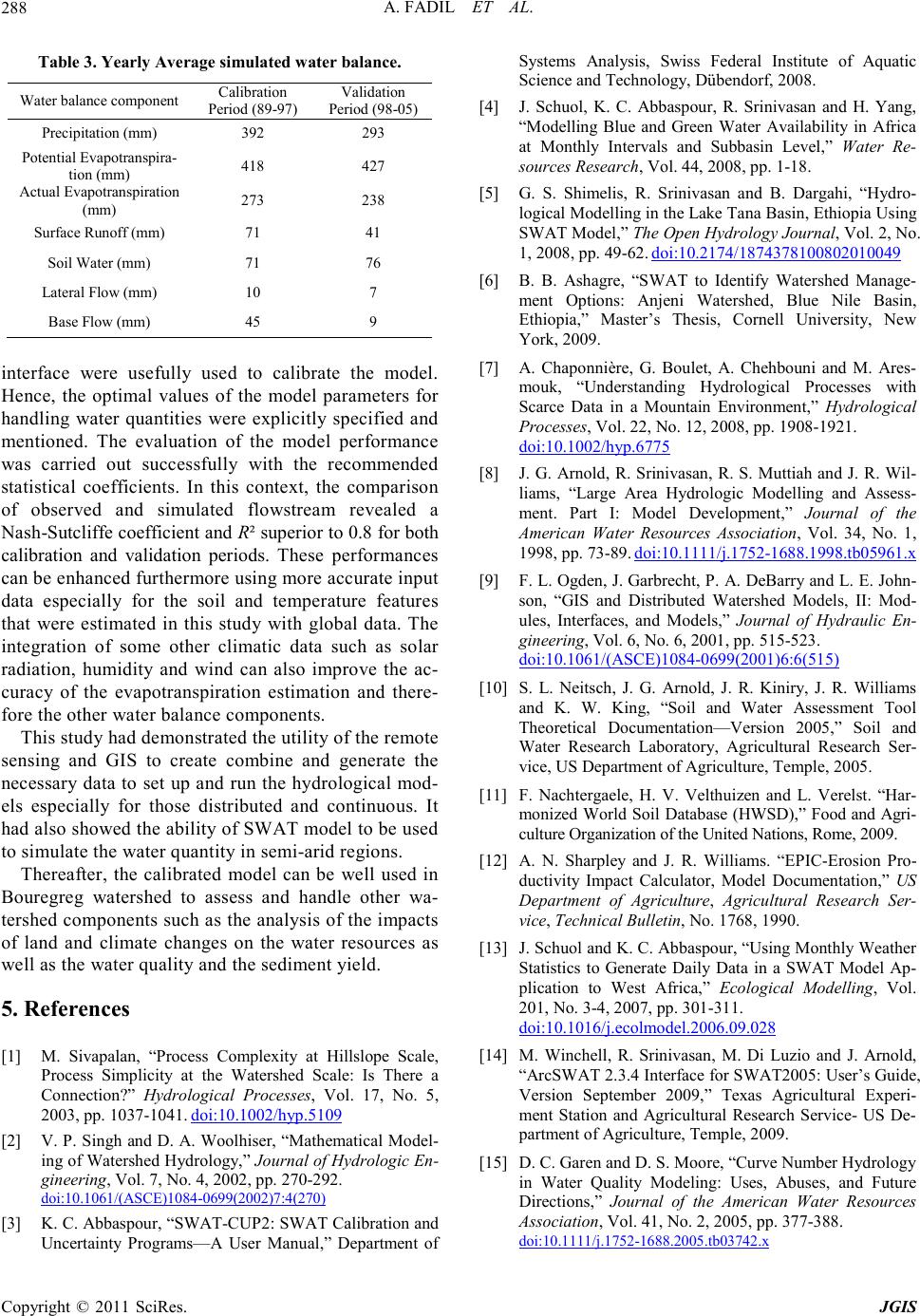
Table 3. Ye ar ly Average simula ted water balance.
Water balance component Calibration
Period (89-97) Validation Period (98-05)
Precipitation (mm) 392 293
Potential E v apotr anspira-
tion (mm ) 418 427
Actual Evapotrans pirati on
(mm) 273 238
Surface Runoff (mm) 71 41
Soil Water (mm) 71 76
Lateral Flow (mm) 10 7
Base Flow (mm) 45 9
interface were usefully used to calibrate the model.
Hence, the optimal values of the model parameters for
handling water quantities were explicitly specified and
mentioned. The evaluation of the model performance
was carried out successfully with the recommended
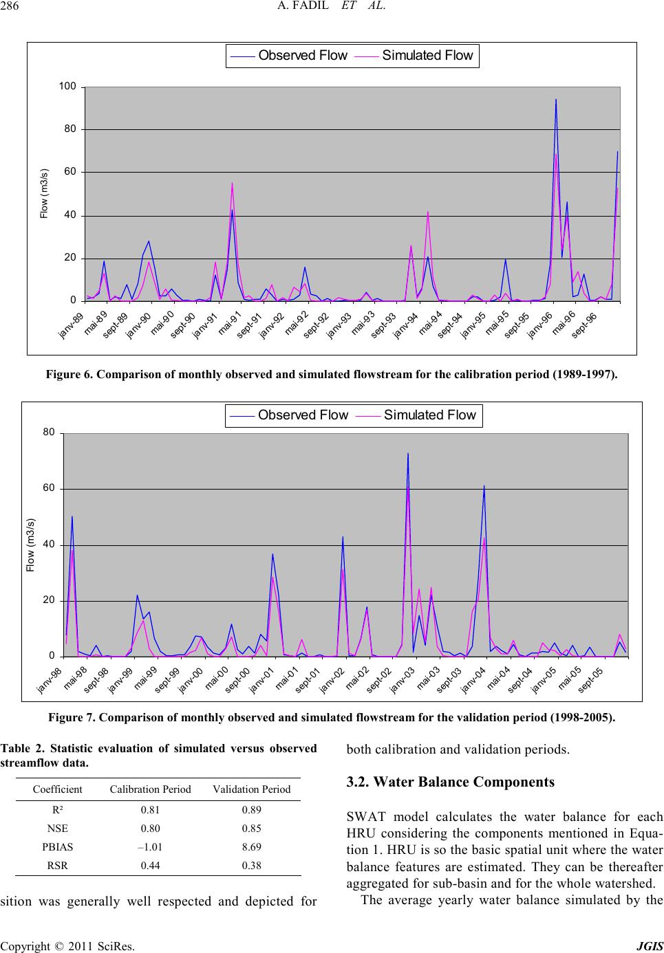
statistical coefficients. In this context, the comparison
of observed and simulated flowstream revealed a
Nas h-Sutcliffe coefficient and R² superior to 0.8 for both
calibration and validation periods. These performances
can be enhanced furt hermore using more accura te input
data especially for the soil and temperature features
that were estimated in this study with global data. The
integration of some other climatic data such as solar
radiation, humidity and wind can also improve the ac-
curacy of the evapotranspiration estimation and there-
fore the other water bala nce co mponents.
This study had demonstrated the utility of the remote
sensing and GIS to create combine and generate the
necessary data to set up and run the hydrological mod-
els especially for those distributed and continuous. It
had also showed the ability of SWAT model to be used
to si mulate t he water quantit y in se mi-arid r e gio ns.
Thereafter, the calibrated model can be well used in
Bouregreg watershed to assess and handle other wa-
tershed components such as the analysis of the impacts
of land and climate changes on the water resources as
well as the water quality and the sediment yield.
5. References
[1] M. Sivapalan, “Process Complexity at Hillslope Scale,
Process Simplicity at the Watershed Scale: Is There a
Connection?” Hydrological Processes, Vol. 17, No. 5,
2003, pp. 1037-104 1. doi:10.1002/hyp.5109
[2] V. P. Singh and D. A. Woolhiser, “Mathematical Model-
ing of Watershed Hydrology,” Journal of Hydrologic En-
gineering, Vol. 7, No. 4, 2002, pp. 270-292.
doi:10.1061 /(ASCE)1084-069 9(2002)7:4(270)
[3] K. C. Abbaspour, “SWAT-CUP2: SWAT Calibration and
Uncertainty Programs—A User Manual,” Department of
Systems Analysis, Swiss Federal Institute of Aquatic
Science and Technology, Dübendorf, 2008.
[4] J. Schuol, K. C. Abbaspour, R. Srinivasan and H. Yang,
“Modelling Blue and Green Water Availability in Africa
at Monthly Intervals and Subbasin Level,” Water Re-
sources Research, Vol. 44, 2008, pp. 1-18.
[5] G. S. Shimelis, R. Srinivasan and B. Dargahi, “Hydro-
logical Modelling in the Lake Tana Basin, Ethiopia Using
SWAT Model,” The Open Hydrology Journal, Vol. 2, No.
1, 2008, pp. 49-62. doi:10.2174/1874378100802010049
[6] B. B. Ashagre, “SWAT to Identify Watershed Manage-
ment Options: Anjeni Watershed, Blue Nile Basin,
Ethiopia,” Master’s Thesis, Cornell University, New
York, 2009.
[7] A. Chaponnière, G. Boulet, A. Chehbouni and M. Ares-
mouk, “Understanding Hydrological Processes with
Scarce Data in a Mountain Environment,” Hydrological
Processes, Vol. 22, No. 12, 2008, pp. 1908-1921.
do i:10.1002/hyp.6775
[8] J. G. Arnold, R. Srinivasan, R. S. Muttiah and J. R. Wil-
liams, “Large Area Hydrologic Modelling and Assess-
ment. Part I: Model Development,” Journal of the
American Water Resources Association, Vol. 34, No. 1,
1998, pp. 73- 8 9. doi:10.1111/j.1752-1688.1998.tb05961.x
[9] F. L. Ogden, J. Garbrecht, P. A. DeBarry and L. E. John-
son, “GIS and Distributed Watershed Models, II: Mod-
ules, Interfaces, and Models,” Journal of Hydraulic En-
gineering, Vol. 6, No. 6, 2001, pp. 515-523.
doi:10.1061/(ASCE)1084-0699(2001)6:6(515)
[10] S. L. Neitsch, J. G. Arnold, J. R. Kiniry, J. R. Williams
and K. W. King, “Soil and Water Assessment Tool
Theoretical Documentation—Version 2005,” Soil and
Water Research Laboratory, Agricultural Research Ser-
vice, US Department of Agriculture, Temple, 2005.
[11] F. Nachtergaele, H. V. Velthuizen and L. Verelst. “Har-
monized World Soil Database (HWSD),” Food and Agri-
culture O rga niza tion of the Unite d Nations , Rom e , 2009.
[12] A. N. Sharpley and J. R. Williams. “EPIC-Erosion Pro-
ductivity Impact Calculator, Model Documentation,” US
Department of Agriculture, Agricultural Research Ser-
vice, Technical Bulletin, No. 1768, 1990.
[13] J. Schuol and K. C. Abbaspour, “Using Monthly Weather
Statistics to Generate Daily Data in a SWAT Model Ap-
plication to West Africa,” Ecological Modelling, Vol.
201, No. 3-4, 2007, pp. 301-311.
doi:10.1016/j.ecolmodel.2006.09.028
[14] M. Winchell, R. Srinivasan, M. Di Luzio and J. Arnold,
“ArcSWAT 2.3. 4 In terface for SWAT2005: User’s Guide,
Version September 2009,” Texas Agricultural Experi-
ment Station and Agricultural Research Service- US De-
partment of Agriculture, Temple, 2009.
[15] D. C. Garen and D. S. Moore, “Curve Number Hydrology
in Water Quality Modeling: Uses, Abuses, and Future
Directions,” Journal of the American Water Resources
Association, Vol. 41, No. 2, 2005, pp. 377-388.
doi:10.1111/j.1752-16 88.2005.tb03 742.x

A. FADIL ET AL. 289
[16] G. Hargreaves and Z. A. Samani, “Reference Crop
Evapotranspiration from Temperature,” Applied Engi-
neering in Agriculture, Vol. 1, No. 2, 1985, pp. 96-99.
[17] R. Rosso, A. Peano, I. Becchi and G. A. Bemporad, “An
Introduction to Spatially Distributed Modelling of Basin
Response,” Water Resources Publications, Highland Ranch,
1994, pp. 3-30.
[18] A. Saltelli, E. M. Scott, K. Chan and S. Marian, “Sensi-
tivity Analysis,” John Wiley & Sons Ltd., Chichester,
2000.
[19] A. Van Griensven and W. Bauwens, “Multi-objective
Auto-calibration for Semi-distributed Water Quality Mod-
els,” Water Resources Research, Vol. 39, No. 12, 2 003.
[20] M. W. Van Liew, J. G. Arnold and D. D. Bosch, “Prob-
lems and Potential of Autocalibrating a Hydrologic
Model,” Transactions of the ASAE, Vol. 48, No. 3, 2005,
pp. 1025 -1040.
[21] K. Beven and A. Binley, “The Future of Distributed
Models—Model Calibration and Uncertainty Prediction,”
Hydrological Processes, Vol. 6, No. 3, 1992, pp. 279-
298. doi:10.1002/hyp.3360060305
[22] A. Van Griensven and T. Meixner, “Methods to Quantify
and Identify the Sources of Uncertainty for River Basin
Water Quality Models,” Water Science and Technology,
Vol. 53, No. 1, 2006, pp. 51-59.
doi:10.2166/wst.2006.007
[23] Q. D. Duan, “Global Optimization for Watershed Model
Calibration,” Water Science Applied Series, Vol. 6, 2003,
pp. 89-1 04. doi :10.1029/WS006 p0089
[24] K. Eckhardt and J. G. Arnold, “Automatic Calibration of
a Distributed Catchment Model,” Journal of Hydrology,
Vol. 251, No. 1-2, 2001, pp. 103-109.
doi:10.1016/S0022-1694(01)00429-2
[25] D. Moriasi, J. G. Arnold, M. W. Van Liew, R. L. Bingner,
R. D. Harmel and T. L. Veith, “Model Evaluation Guide-
lines for Systematic Quantification of Accuracy in Wa-
tershed Simulations,” Transactions of the ASABE, Vol.
50, No. 3, 200 7 , pp. 885-900 .
[26] J. E. Nash and J. V. Sutcliffe, “River Flow Forecasting
through Conceptual Models, Discussion of Principles,”
Journal of Hydrology, Vol. 10, No. 3, 1970, pp. 282-290.
do i:10.1016/ 0022- 1694(70)90 255-6
[27] H. V. Gupta, S. Sorooshian and P. O. Yapo, “Status of
Automatic Calibration for Hydrologic Models: Compari-
son with Multilevel Expert Calibration,” Journal of Hy-
drologic Engineering, Vol. 4, No. 2, 1999, pp. 135-143.
doi:10.1061/(ASCE)1084-0699(1999)4:2(135)
[28] J. Singh, H. V. Knapp and M. Demissie, “Hydrologic
Modeling of the Iroquois River Watershed Using HSPF
and SWAT,” Journal of the American Water Resources
Association, Vol. 41, No. 2, 2004, pp. 343-360.
doi:10.1111/j.1752-1688.2005.tb03740.x
[29] K. L. White and I. Chaubey, “Sensitivity Analysis, Cali-
bration, and Validations for a Multisite and Multivariable
SWAT Model,” Journal of the American Water Resources
Association, Vol. 41, No. 5, 2005, pp. 10 77-1089.
doi:10.1111/j.1752-1688.2005.tb03786.x