Journal of Electromagnetic Analysis and Applications
Vol. 2 No. 5 (2010) , Article ID: 1921 , 13 pages DOI:10.4236/jemaa.2010.25043
Progressing of Quantum Tomography for Quantum Information Acquisition*
![]()
Department of Automation, University of Science and Technology of China, Hefei, China.
Email: chenzh@ustc.edu.cn
Received September 5th, 2009; revised November 8th, 2009; accepted November 21st, 2009.
Keywords: Quantum Tomography, Quantum Information Acquisition, Quantum State Estimation, Review and Expectation
ABSTRACT
In this paper we review a number of recent developments in the study of quantum tomography which is one of the useful methods for quantum state estimation and quantum information acquisition, having sparked explosion of interest in recent years. The quantum process tomography is also analyzed. At the same time, some success experiments and applications of quantum tomography are introduced. Finally, a number of open problems and future directions in this field are proposed.
1. Introduction
In the past few years, quantum tomography has attracted considerable attention as well as experimental research. Much of this work has already been summarized in several reviews [1-6].
The state of a physical system is the mathematical description of our knowledge of it. If we can acquire the state we’ll get complete information on its past and future. The knowledge of the state is equivalent to know the result of any possible measurement on the system. A state estimation technique is a method that provides the complete description of a system, thus allowing one to make at least the best predictions on the results of any measurement that may be performed on the system. In classical physics it is always possible, at least in principle, to devise a procedure that fully recovers the state of a system. But, in Quantum Mechanics this is no longer possible, and this impossibility is inherently related to fundamental features of the theory, such as the Heisenberg uncertainty principle and no-cloning theorem. On one hand, the no-cloning theorem [7] forbids us to create perfect copies of an unknown state in order to make different measurements on the same state. On the other hand, the Heisenberg uncertainty principle [8] indicates that one cannot perform an arbitrary sequence of measurements on a single system without disturbing it in some way. Therefore, it is not possible, even in principle, to determine the quantum state of a system without any prior knowledge on it [9]. This is consistent with the very definition of a quantum mechanical state, which prescribes how to gain information about the state: for a quantum mechanical system it is possible to estimate the unknown state of a system when many identical preparations taken from the same statistical ensemble are available, so that a different measurement can be performed on each of the copies. A procedure of this kind is called Quantum Tomography (QT), which is described as an inverse statistical problem in which the quantum state of a system is the unknown parameter and the data are given by the results of measurements performed on identical quantum states [4]. The quantum state can be represented as an infinite dimensional density matrix. Thus, one can acquire information about the state by reconstructing the density matrix ρ.
The first systematic approach for inferring state of a quantum system was U. Fano’s work in the late fifties of last century. [10] In the last decade a constantly increasing interest has been devoted to the subject. On one side, new developments in experimental techniques, especially in the fields of photodetection and nonlinear optics, resulted in a set of novel and beautiful experiments about quantum mechanics. On the other side, increasing attention has been directed to quantum information technology, such as error correction, purification, fault tolerant quantum computing, long distance teleportation and cryptography. In particular, a characterization of quantum channels relies heavily on quantum tomography techniques. Tomographic methods were initially employed only for measuring radiation states. However, they can profitably be used also to characterize devices through characterization of quantum operations performed on quantum states. This process is called Quantum Process Tomography (QPT) [11-13].
In quantum process tomography, a device of some sort repeatedly prepares many instances of a quantum system in a fixed quantum state ρ. An experimentalist who wishes to characterize the operation of the device or to adjust it for future use may be able to perform measurements on the systems it prepares. He lets an incompletely specified device act on a quantum system prepared in an input state by his choice, and then performs a measurement on the output system. This procedure is repeated many times, with possibly different input states and different measurements, in order to accumulate enough statistics to assign a quantum operation to the device. Then learning about the state will also be learning about the device. The goal of the experimenter is to perform enough measurements, namely enough kinds of measurements on a large enough sample, to estimate ρ and characterize operation of the device. All the operations we mentioned in this paper are trace-preserving completely positive linear map.
Basing on the results of theoretical research, a few experimentalists began to enter the realm of experiment of quantum tomography and quantum process tomography, and the first experiments performed by Michael Raymer’s group at the University of Oregon [14-15], which already showed the results for reconstructions of coherent and squeezed states. In the next decade, there is a quick emergence of many experiments results [2,16-25]. The first exact technique was given for measuring experimentally the matrix elements of the density operator in the photon-number representation [26] by simply averaging functions of homodyne data. After that, the method was further simplified [27], and the feasibility for non-unit quantum efficiency of detectors above some bounds was established. The exact homodyne method has been implemented experimentally to measure the photon statistics of a semiconductor laser [28], and the density matrix of a squeezed vacuum [29]. The success of optical homodyne tomography has then stimulated the development of state-reconstruction procedures for atomic beams [30], the experimental determination of the vibrational state of a molecule [31], of an ensemble of helium atoms [32], and of a single ion in a Paul trap [33]. Thus, the utility of these theories has been verified by relevant experiments. Meanwhile, quantum process tomography has been demonstrated experimentally in liquid state nuclear magnetic resonance [24,34], and recently a number of optical experiments [35-36] have implemented entanglement assisted quantum process tomography. In the third section some important scheme and results about experiments are specified.
This paper aims to review the chief relevant theory and techniques about quantum tomography which has provoked renewed interest in fundamental quantum mechanics. It will consist of two major sections. The first presents the general theory about quantum tomography and quantum process tomography; the second illustrates some experiments and application about them. Finally, a number of challenges for future work are summarized. A number of leading experts have cooperated to describe the main features in this novel field. We will attempt to proceed in a constructive way, making connections with previously presented notions and techniques when possible. If this paper can make more relevant researchers pay attention to these we’ll feel gratified.
2. Quantum Tomographic Methods
What is quantum state? The interpretation, well stated by Leonhardt, is that “knowing the state means knowing the maximally available statistical information about all physical quantities of a physical object”. Typically by “maximally available statistical information” we mean probability distributions. Hence, knowing the state of a system means knowing the probability distributions corresponding to measurements of any possible observable pertaining to that system. Since knowing the state means knowing all the statistical information about a system, is the inverse true? If one knows all of the statistical information about a system, does one then know the quantum state of that system? Clearly, a real experiment cannot measure all possible statistical information. A more practical question is then: can one infer reasonably well the quantum state of a system by measuring statistical information corresponding to a finite number of observables?
The answer to this question is a resounding yes. But there are some caveats. By now it is well established that the state of an individual system cannot, even in principle, be measured [37]. This is easily seen by the fact that a single measurement of some observable yields a single value, corresponding to a projection of the original state onto an eigenstate that has nonzero probability. Clearly this does not reveal much information about the original state. This same measurement simultaneously disturbs the individual system being measured, so that it is no longer in the same state after the measurement. This means that subsequent measurements of this same system are no longer helpful in determining the original state.
Since state measurement requires statistical information, multiple measurements are needed, each of which disturbs the system being measured. Here each member of an ensemble of systems is prepared by the same statepreparation procedure. Each member is measured only once, and then discarded. Thus, multiple measurements can be performed on systems all in the same state, without worrying about the measurement apparatus disturbing the system. A mathematical transformation is then applied to the data in order to reconstruct, or infer, the state. The relevant interpretation of the measured state in this case is that it is the state of the ensemble. Because in quantum state measurement the collected data is analyzed using a mathematical technique that is very similar to the tomographic reconstruction technique used in medical imaging, and because all techniques are necessarily indirect, a generally accepted term for quantum state measurement has become Quantum State Tomography, for short, quantum tomography. The aim of quantum tomography is to reconstruct the density matrix of quantum states. Some relevant theories are introduced in the following section.
2.1 General Theory of Quantum Tomography
2.1.1 Wigner Function
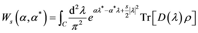
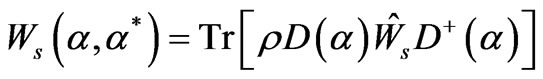
As a method to express the density operator in terms of c-number functions, the Wigner functions often lead to considerable simplification of the quantum equations of motion. Using the Wigner function one can express quantum-mechanical expectation values in form of averages over the complex plane (the classical phase-space), where the Wigner function playing the role of a c-number quasi-probability distribution, which generally can also have negative values. More precisely, the original Wigner function allows us to easily evaluate expectations of symmetrically ordered products of the field operators. However, with a slight change of the original definition, one defines generalized s-ordered Wigner function  as follows [38]:
 (1)
(1)
where  denotes the complex conjugate of
![]() , the integral is performed on the complex plane with measure
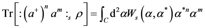
, the integral is performed on the complex plane with measure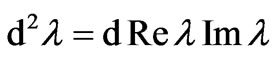 , ρ represents the density operator. The Wigner function in (1) allows one to evaluate s-ordered expectation values of the field operators through the following relation:
 (2)
(2)
The particular cases  correspond to antinormal, symmetrical, and normal ordering, respectively. In these cases the generalized Wigner function
  are usually denoted by the following symbols and names:
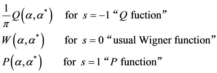 (3)
(3)
For the normal (s = 1) and anti-normal (s = −1) orderings, the following simple relations with the density matrix are well known:
 (4)
(4)
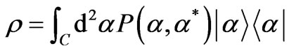 (5)
(5)
where 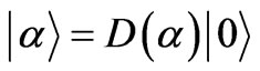 and
and  is the vacuum state of the field. The usual Wigner function has the remarkable property of providing the probability distribution of the quadratures of the field in the form of a marginal distribution, namely:
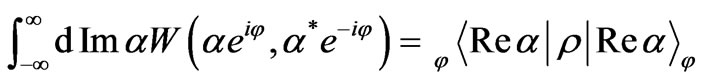 (6)
(6)
where  denotes the eigenstate of the field quadrature:
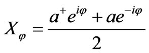 (7)
(7)
with real eigenvalues x. Notice that any couple of quadratures is canonically conjugate, namely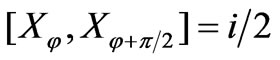 , and it is equivalent to position and momentum of a harmonic oscillator. From (1) one can notice that all s-ordered Wigner functions are related to each other through Gaussian convolution:
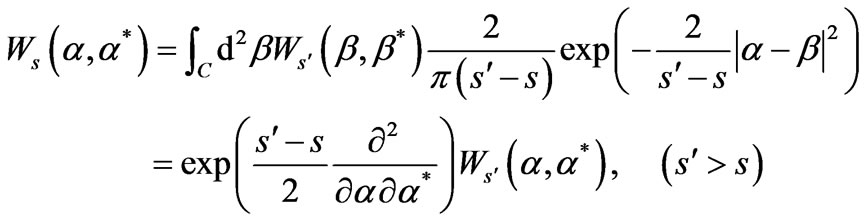 (8)
(8)
Equation (8) shows the positivity of the generalized Wigner function for , as a consequence of the positivity of the Q function. The maximum value of s keeping the generalized Wigner functions as positive can be considered as an indication of the classical nature of the physical state [39].
An equivalent expression for  can be derived as follows. Equation (1) can be rewritten as:
 (9)
(9)
Where,
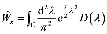 (10)
(10)
Thus, the density matrix can be recovered from the generalized Wigner functions and, in particular, for s = 0 one has the inverse of the Glauber formula:
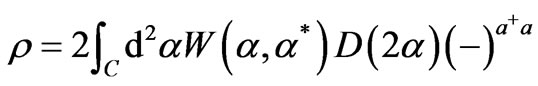 (11)
(11)
whereas, for s = 1, ![]() can be recovered according to (5).
can be recovered according to (5).
2.1.2 Balance Homodyne Detection [14,40-41]
The balanced homodyne detector provides the measurement of the quadratures of the field  in (7). It was proposed by Yuen and Chan [42], and subsequently demonstrated by Abbas, Chan and Yee [43].
The scheme of a balanced homodyne [27,44] detector is depicted in Figure 1. The signal mode a interferes with a strong laser beam mode b in a balanced 50/50 beam splitter. The mode b is so-called local oscillator (LO) mode of the detector. It operates at the same frequency of a, and is excited by the laser in a strong coherent state . Since in all experiments that use homodyne detectors the signal and the LO beams are generated by a common source, we assume that they have a fixed phase relation. In this case the LO phase provides a reference for the quadrature measurement, namely, we identify the phase of the LO with the phase difference between the two modes. As we will see, by tuning
 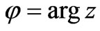 we can measure the quadratures
  at different phases. After the beam splitter the two modes are detected by two identical photodetectors (usually linear avalanche photodiodes), and finally the difference of photocurrents at zero frequency is electronically processed and rescaled by
 , the modes at the output of the 50/50 beam splitter are written:
 (12)
(12)
hence the difference of photocurrents is given by the following operator:
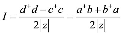 (13)
(13)
Thus, the probability distribution of the output photocurrent I for a generic state ρ of the signal mode a can be evaluated.
2.2 Qubit Quantum Tomography [5,45-47]
Much like its classical counterpart, which aims at reconstructing three-dimensional images via a series of twodimensional projections along various ‘cuts’, quantum tomography characterizes the complete quantum state of a particle through a series of measurements in different bases. While the characterization of a classical object can perform a series of measurements on the same subject, measuring a single quantum particle disturbs its state, often making its further investigation uninformative. For this reason, quantum tomography must be carried out on a number of identical copies of the same state separately.
Before states can be analyzed, it is necessary to understand their representation. In particular, the reconstruction of an unknown state is often simplified by a specific state parametrization. In general, any single-qubit in a
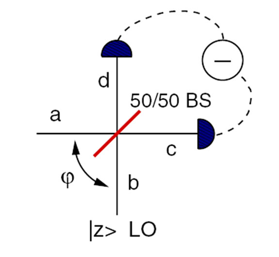
Figure 1. Scheme of balance homodyne detector
pure state can be represented by:
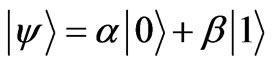 (14)
(14)
where ![]() and
and  are complex and
  [48]. If the normalization is written implicitly and the global phase is ignored, this can be rewritten as:
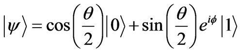 (15)
(15)
These representations are sufficient to enable the description of the action of any operator (e.g., projectors or unitary rotations) on a pure state, and therefore to carry out tomography on that state. Meanwhile, mixed states may be described by a probabilistically weighted incoherent sum of pure states. In other words, it is as if any particle in the ensemble has a specific probability of being in a given pure state, and this state is distinguishably labeled in some way. A mixed state can be represented by a density matrix :
:
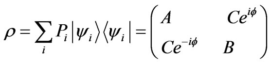 (16)
(16)
While any ensemble of pure states can be represented in this way, it is also true that any ensemble of singlequbit states can be represented by an ensemble of only two orthogonal pure states. Any physical density matrix can be diagonalized, such that:
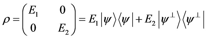 (17)
(17)
where 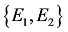 are the eigenvalues of
 , and
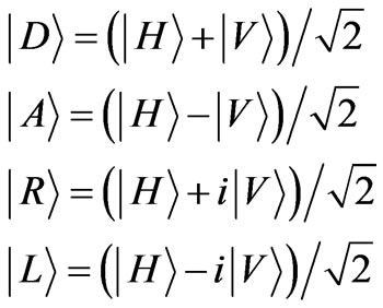
, and 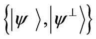 are the eigenvectors. Thus the representation of any quantum state, no matter how it is constructed, is identical to that of an ensemble of two orthogonal pure states [49]. For example, order horizontal
 , vertical
 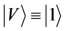 and
and
 (18)
(18)
then
 (19)
(19)
which, as predicted, is a sum of only two orthogonal states. In particular, any single-qubit density matrix  can be uniquely represented by four Stokes parameters
 :
:
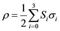 (20)
(20)
where,
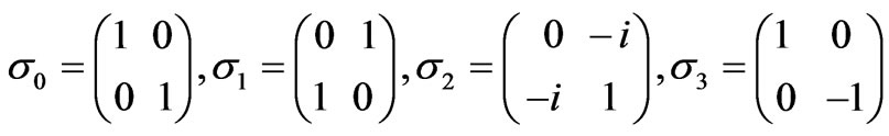 (21)
(21)
and the  values are given by:
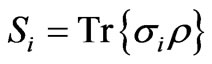 (22)
(22)
For all pure states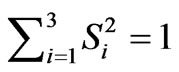 ; for mixed states
 ; for the completely mixed state
 . Due to normalization,
  will always equal one.
Although reconstructive tomography of any size system follows the same general procedure, beginning with tomography of a single qubit allows the visualization of each step using the Block Sphere, in addition to providing a simpler mathematical introduction. Exact singlequbit tomography requires a sequence of three linearly independent measurements. Each measurement exactly specifies one degree of freedom for the measured state, reducing the free parameters of the unknown state’s possible Hilbert space by one.
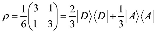
As an example, consider measuring ,
,  and
and  on the mixed state:
 (23)
(23)
This form allows us to read off the normalized Stokes parameters corresponding to these measurements:
 (24)
(24)
As always,  due to normalization. Measuring R first, and looking to the Block Sphere, we see that the unknown state must lie in the
  plane (
 ). A measurement in the D basis further constrains the state to the y = 0 plane (
 ), resulting in a total confinement to a line parallel directly above the x axis. The final measurement of H pinpoints the state to the
  plane (
 ). This process is illustrated in Figure 2. Obviously the order of the measurements is irrelevant: it is the intersection point of three orthogonal planes that defines the location of the state.
If instead measurements are made along non-orthogonal axes, a very similar picture develops, as indicated in Figure 3. The first measurement always isolates the unknown state to a plane, the second to a line, and the third to a point.
Of course, in practice, the experimenter has no knowledge of the unknown state before a tomography. The set of the measured probabilities, transformed into the Stokes parameters as above, allow a state to be directly reconstructed.
2.3 Quantum Process Tomography
In quantum process tomography [11-13], an experimenter lets an specified device act on a quantum state prepared in an input state by his choice, and then performs a measurement on the output state. This procedure is repeated many times for different input states and different measurements, in order to accumulate enough statistics to assign a quantum operation to the device. In fact quantum
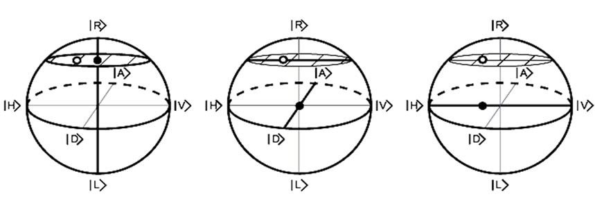
Figure 2. [5] A sequence of three linearly independent measurements isolates a single quantum state in Hilbert space (shown here as an open circle in the Block Sphere representation)
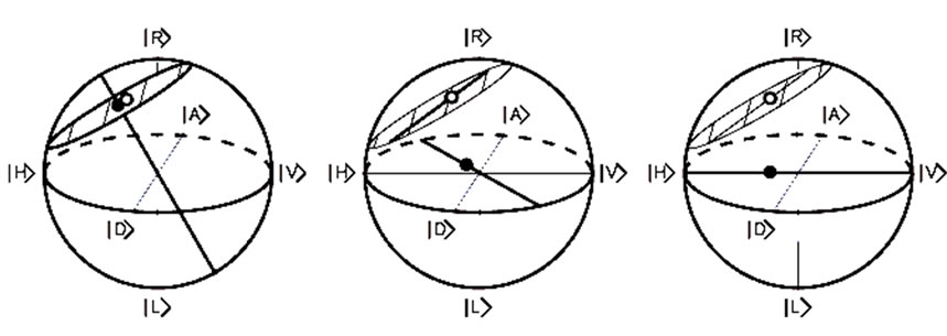
Figure 3. [5] A sequence of measurements on the same state taken using non-orthogonal projections: elliptical light rotated  from H towards R,
  linear, and horizontal
process tomography is equivalent to quantum state tomography in a larger state space [50].
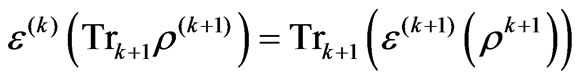
In the usual description of process tomography, it is assumed that the device performs the same unknown quantum operation ![]() every time, and an experimenter’s prior information about the device is expressed via a probability density p (ε). Here, we restrict our attention to devices for which the input and output have the same Hilbert space dimension D.
every time, and an experimenter’s prior information about the device is expressed via a probability density p (ε). Here, we restrict our attention to devices for which the input and output have the same Hilbert space dimension D.  denotes a D-dimensional Hilbert space,
  denotes its N-fold tensor product and L (V) denotes the space of linear operators on a linear space V. The set of density operators for a D-dimensional quantum system is a convex subset of
 . The action of a device on inputs state is then described by a trace-preserving completely positive map:
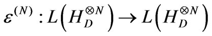 (25)
(25)
which maps the input state to the output states. In analogy to the definition of exchangeability for quantum states, a quantum operation  is exchangeable if it is a member of an exchangeable sequence of quantum operations.
Any N-system density operator  can be expanded in the form:
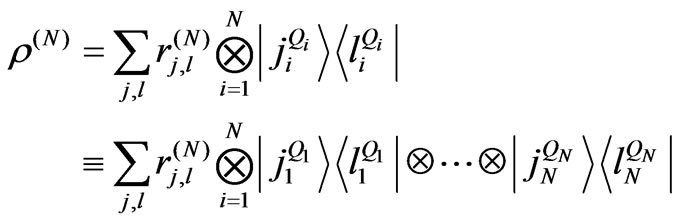 (26)
(26)
where 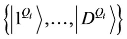 denotes an orthonormal basis for the Hilbert space
  of the ith state, and
  are the matrix elements of
  in the tensor product basis. We define the action of the permutation π on the state
  by:
by:
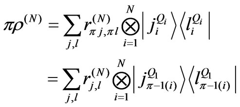 (27)
(27)
With this notation, we can make the following definition. A sequence of quantum operations, 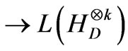
 , is called exchangeable. For
 1)
1)  is symmetric, i.e.,
 (28)
(28)
for any permutation π of the set  and for any density operator
 .
.
2)  is extendible, i.e.,
 (29)
(29)
for any state .
.
In words, these conditions amount to the following. Condition (1) indicates the requirement that the quantum operation  commutes with any permutation operator π acting on the state
 : It does not matter what order the states are sent through the device; as long as they are rearranged into the original order at the end, the resulting evolution will be the same. Condition (2) says that it does not matter if we consider a larger map
  acting on a larger collection of states, or a smaller
  on some subset of those states: The upshot of the evolution will be the same for the relevant states.
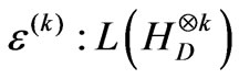
A quantum operation 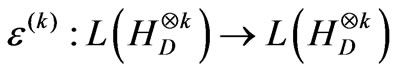 is an element of an exchangeable sequence if and only if it can be written in the form:
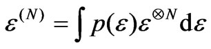 for all N(30)
where the integral ranges over all single-shot quantum operations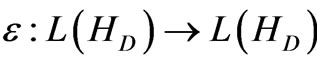 ,
,  is a suitable measure on the space of quantum operations, and the probability density
  is unique. The tensor product
  is defined by
  for all
  and by linear extension for arbitrary arguments.
This result allows certain latitude in how quantum process tomography can be described. One is free to use the language of an unknown quantum operation if the condition of exchangeability is met by one’s prior  but it is not required: in particular, the known quantum operation
  is the only meaningful quantum operation in the problem. The proof of the process tomography theorem is specified in this book [6].
2.4 Error Analysis [51]
Error analysis of reconstructed density matrices is in practice a non-trivial process. The traditional method of error analysis involves analytically solving for the error in each measurement due to each source of error, then propagating these errors through a calculation of any derived quantity. In the photon case, for example, errors in counting statistics are analyzed [52], giving errors in both density matrices and commonly derived quantities, such as the tangle and the linear entropy. In practice, however, these errors appear to be too large: In [52]measurements had been repeated many times, and observed a spread in the value of derived quantities which is approximately an order of magnitude smaller that the spread predicted from an analytic calculation of the uncertainty. Thus it is worthwhile to discuss alternate methods of error analysis.
One promising numerical method is the ‘Monte Carlo’ technique, whereby additional numerically simulated data is used to provide a statistical distribution over any derived quantity. Once an error distribution is understood over a single measurement, a set of ‘simulated’ results can be generated. These results are simulated using the known error distributions in such a way as to produce a full set of numerically generated data which could feasibly have come from the same system. Many of these sets of data are numerically generated (at the measured counts level), and each set is used to calculate a density matrix via the maximum likelihood technique [40,53-56]. This set of density matrices is used to calculate the standard error on any quantity implicit in or derived from the density matrix.
As an example, consider the application of the Monte Carlo technique to the down-conversion results [57]. Two polarization encoded qubits are generated within ensembles that obey Poisson statistics, and these ensembles are used to generate a density matrix using the maximum likelihood technique [40,55-56]. In order to find the error on a quantity derived from this density matrix, 36 new measurement results are numerically generated, each drawn randomly from a Poisson distribution with mean equal to the original number of counts. These 36 numerically generated results are then fed into the maximum likelihood technique, in order to generate a new density matrix, from which, the tangle may be calculated. This process is repeated many times, generating both many density matrices and a distribution of tangle values, from which the error in the initial tangle may be determined. In practice, additional sets of simulated data must be generated until the error on the quantity of interest converges to a single value.
Clearly, the problem of error analysis in state tomography is an area of continuing research. The developpment of adaptive tomography techniques could allow both specific measurements and the data collection times to be reduced in order to optimize for each state to be measured. In addition, because the number of measurements necessary to perform grows exponentially with the number of qubits, it will eventually be necessary to partially characterize states with fewer measurements. Finally, each distinct qubit implementation provides a myriad of unique challenges. Nevertheless, the discussions presented here will be useful for characterizing quantum systems in a broad spectrum of qubit realizations.
3. Research on Experiments
In order to verify the correction of the theory, many experimenters began to focus on the research on experiment and there were more and more satisfying results emerging. The theoretical efforts were complemented by a number of important experimental works suggesting the feasibility and importance of quantum tomography.
The first exact technique was given for measuring experimentally the matrix elements of the density operator in the photon-number representation [26] by simply averaging functions of homodyne data. After that, the method was further simplified [27], and the feasibility for non-unit quantum efficiency of detectors above some bounds was established. The exact homodyne method has been implemented experimentally to measure the photon statistics of a semiconductor laser [28], and the density matrix of a squeezed vacuum [29]. The success of optical homodyne tomography has then stimulated the development of state-reconstruction procedures for atomic beams [30], the experimental determination of the vibrational state of a molecule [31], of an ensemble of helium atoms [32], and of a single ion in a Paul trap [33]. In this section some experiments about quantum tomography and quantum process tomography are introduced.
3.1 An Example: Density Matrix Reconstruction in NMR [58-59]
In NMR quantum computation, the liquid ensemble is described by the density matrix. The state of the NMR computer can be obtained by the state-tomography technique [60]. In order to extract the density matrix, for example, for a 2-qubit system, for a 2-qubit system, 18 read-outs have to be performed. In general, for an n-qubit system, construction of the density matrix requires  read-outs. After signal readout, the area of the spectrum is integrated and the density matrix is reconstructed through numerical methods. Obviously, the amount of work in experiment is huge when n becomes moderately large. So, in practice, when n is small the scheme is feasible.
In an NMR measurement, each read-out pulse can only give some off-diagonal matrix elements of the density matrix. To obtain the rest of the matrix elements, one has to rotate the original density matrix through rotational operations. For a 2-qubit system, in order to construct the density matrix, one needs to perform the following operations: II, IX, IY, XI, XX, XY, YI, YX and YY. Here, I, X and Y stand for, respectively, the identity operation, a 90◦ rotation about the x-axis, and a 90◦ rotation about the y-axis.
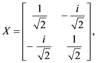
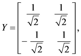
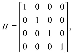
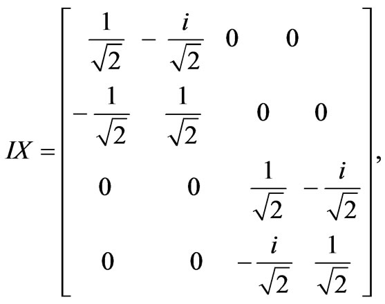
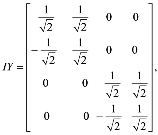
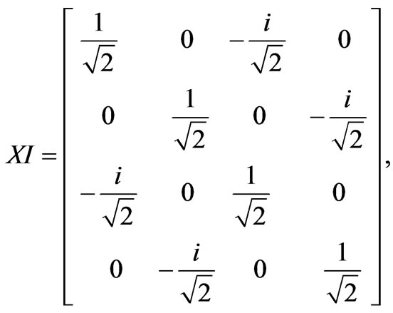
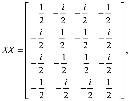
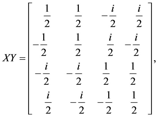
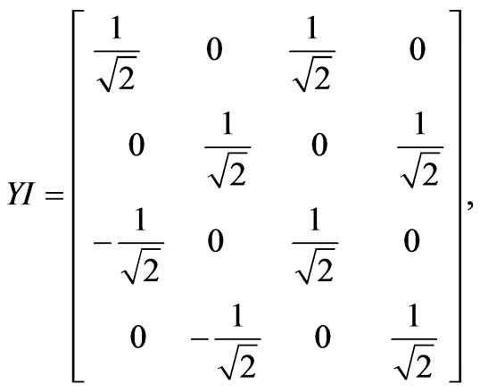
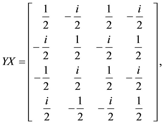
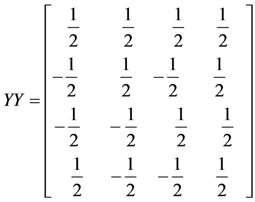
Thus, in a quantum state tomography, these operations are performed before NMR measurements. Suppose that the nuclear spins of H and P in a phosphorous acid are used for qubits. For a usual NMR system, only one nuclear spin can be measured at a time, the measurement has to be performed separately for the two nuclear spins, H and P. Next, we restart the computation, but this time the operation IX is performed at the required state before measurement. This process is carried out separately for H and P nuclear spins, and the nine operations are successively performed on each of them. This means that 9 × 2 = 18 read-outs are acquired. Suppose the density matrix is following form:
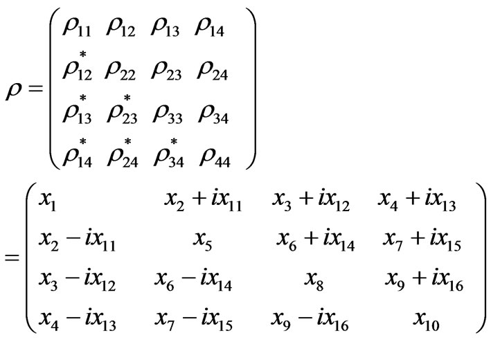 (31)
(31)
The NMR read-out signal can only give  and
and  from the nuclear spin of P, and
  and
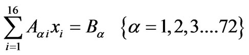
and  from the nuclear spin of H. To obtain other elements in the density matrix, one of the nine operations is performed on the state so that the desired elements are transformed to the positions which can be given by read-out. Altogether, 4 × 9 × 2 = 72 equations with 16 unknowns are obtained:
 (32)
(32)
namely:
 (33)
(33)
There are certainly redundant expressions in (32) since the number of equations is more than the number of unknowns. The standard way of dealing with this problem is to use the least-square-fitting procedure which is widely used in various problems in science and engineering. We minimize the quantity  defined as:
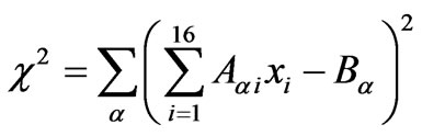 (34)
(34)
To find the minimum, a variation procedure on  with respect to all parameters is carried out, which gives:
 (35)
(35)
here,  ,
, . According to
 , the formula (35) becomes:
 (36)
(36)
Here,  ,
,  , U is the unitary matrix which diagonalizes C, Cd is diagonal matrix.[61] So, the equation becomes:
 (37)
(37)
According to Y we can acquire the Y. Thus, the density matrix is constructed.
3.2 Quantum Process Tomography Applied in Quantum Channel
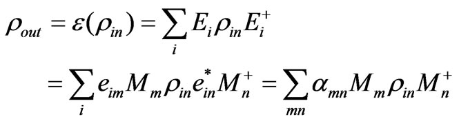
In quantum communication, when the state  pass through the quantum channel the physical transformation can be described by a super-operator
![]() . The process can be formulized
. The process can be formulized
 (38)
(38)
Basing on the relationship between the input and output the super-operator can be characterized as in Figure 5.
Because of physical reasonability, the super-operator must accord with the following three characters: trace-preserving, positivity, and linearity. Then, (38) can be rewritten
 (39)
(39)
where,  ,
,  is the presentation of Kraus operator.
While the operator cannot be measurement directly in physics, the super-operator, ![]() , which represents the character of quantum channel must be parameterized. The Kraus operator,
, which represents the character of quantum channel must be parameterized. The Kraus operator,  is represented by a set of basis
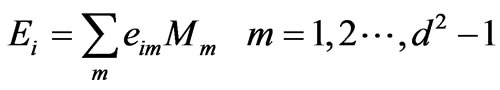 (40)
(40)
where, ![]() is the dimension of the input quantum state. So we get
is the dimension of the input quantum state. So we get
 (41)
(41)
where,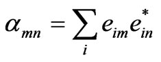 .
.
From above format we know that acquiring the matrix ![]() is equivalent to characterizing the quantum channel. Matrix
is equivalent to characterizing the quantum channel. Matrix ![]() has different form according to choice of the
has different form according to choice of the
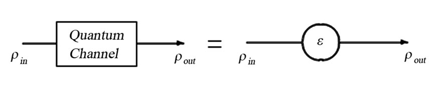
Figure 4. In the process of quantum states passing through quantum channel, the information about a quantum channel is encoded in the state
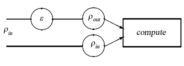
Figure 5. The scheme for characterizing the super-operator ![]() which performed on quantum state passing through the quantum channel
which performed on quantum state passing through the quantum channel
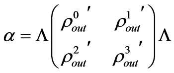
basis. For example, we choose 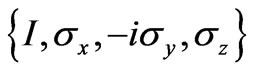 as the basis
 , then
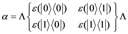 (42)
(42)
where, 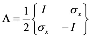 , d = 2.
Let the input states 
 pass through the quantum channel and measure the corresponding output states
 . Then the matrix
 ![]() can be obtained according to (42). It is noticeable that the density matrix such as
can be obtained according to (42). It is noticeable that the density matrix such as  is illegal. Luckily, they can be calculated indirectly because super operator is linear
 (43)
(43)
Where,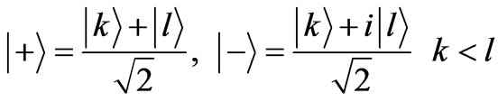 .
.
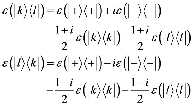
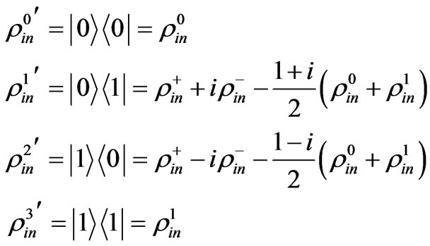
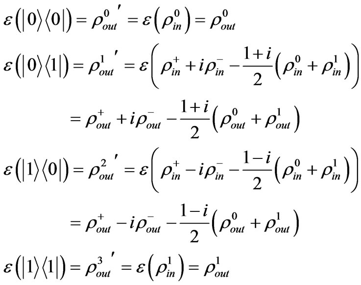
The polarization state of a photon is a natural experimental realization of a two-level quantum system-a qubit. In following section, an experiment scheme in which the polarization state of photon is selected for experimental object is demonstrated. We choose the input states
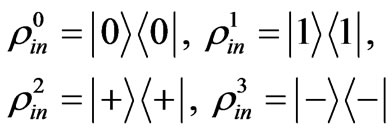 (44)
(44)
where, 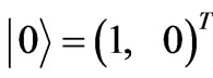 ,
,  ,
,  ,
, .
.
The density matrix of output state is acquired by following steps:
1) Let a large number of output photons from quantum channel pass through the vertical-polarization waveplate and record the number at back: ;
;
2) Let a large number of output photons from quantum channel pass through the horizontal-polarization waveplate and record the number at back: ;
;
3) Let a large number of output photons from quantum channel pass through the left-rotation waveplate and record the number at back: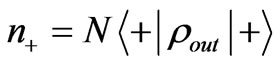 ;
;
4) Let a large number of output photons from quantum channel pass through the right-rotation waveplate and record the number at back: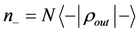 .
.
The density matrix of output photon is reconstructed according to ( ,
,  ,
,  ,
, ):
):
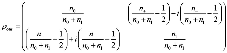 (45)
(45)
by this mean, the corresponding output density matrixes for input,  ,
,  ,
,  ,
,  are obtained,
  ,
,  ,
,  ,
,  , after that, the needed transforms are made:
 (46)
(46)
corresponding transforms on output density matrixes:
 (47)
(47)
Finally, the parameter matrix ![]() on the basis
on the basis 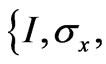
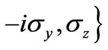 is achieved:
 (48)
(48)
4. Conclusions and Future Challenges
The state of a physical system is the mathematical object that provides complete information on the system. The knowledge of the state is equivalent to know the result of any possible measurement on the system. Quantum tom-
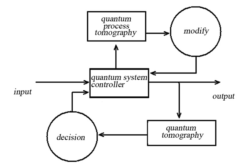
Figure 6. The design of quantum feedback control system using quantum tomography for quantum information acquisition
ography offers a method to estimate a generic quantum system from the measurement of a suitable set of observables, a quorum, on repeated preparations of the system.
Quantum state tomography has come of age. Many theoretical methods exist for converting measured results into information for the quantum state. Numerous experiments demonstrating the utility of these theories have been performed. These experiments have used several different detection technologies, and have measured various quantities ranging from Wigner functions to photon number and phase distributions. According to the characters of quantum tomography, there will be some expectant applications as fellow:
4.1 Preparation of Quantum States
For many experiments in quantum theory and quantum information it is very important to develop reliable sources of arbitrary polarization quantum states. Quantum tomography is important for the development of new quantum sources, since the quantum state reconstruction techniques are natural means of calibration and tuning of experimental apparatuses.
4.2 Quantum Information Acquisition and Characterization of Control System in Quantum Control System
In classical control, the information acquisition and feedback are very important concept. But, in quantum control system, the carrier of information is the quantum states and information is encoded in it. The state, however, is not an observable in quantum mechanics [62] and, thus, a fundamental problem arises: the desired transformation is performed on the input state by the quantum system controller, then, the information has to be read out, in other words, the output state has to be determined in order to judge the performance of control system and make new decision for following action. In quantum control system there is anther problem: the parameters of controller are not exact, so we must try to find out and modify them according to our demand.
In some ways, quantum tomography can solve above problem. Figure 6 shows that the output state can be determined by quantum tomography that assists to change control strategy better; the parameters of controller are obtain from quantum process tomography at the necessary time and one is able to modify them on his demand. Thus, the quantum system will evolve at the desired direction. The work in this area is really just beginning, and we expect it to have a bright future.
REFERENCES
- G. M. D’Ariano, “Quantum Tomography: General Theory and New Experiments,” Fortschr Phys, Vol. 48, No. 5-7, 2000, pp. 579-588.
- G. M. D’Ariano, M. D. Laurentis, et al., “Quantum Tomography as a Tool for the Characterization of Optical Devices,” Journal of Optics B: Quantum and Semiclassical Optics, Vol. 4, No. 3, 2002, pp. S127-S132.
- G. M. D’Ariano, M. G. A. Paris and M. F. Sacchi, “Quantum Tomography,” Advances in Imaging and Electron Physics, Academic Press Inc., Vol. 128, 2003, pp. 205- 308.
- L. M. Artiles, R. D. Gill and M. I. Guta, “An Invitation to Quantum Tomography,” Journal of the Royal Statistical Society Series B, Vol. 67, No. 1, 2005, pp. 109-134.
- Z. Hradil, J. Rehacek, et al., “Qubit Quantum State Tomography,” Lecture Notes in Physics, Vol. 649, 2004, pp. 113–145.
- M. G. A. Paris and J. Rehácek, “Quantum State Estimation,” Springer, Berlin, 2004.
- W. K. Wootters and W. H. Zurek, “A Single Quantum cannot be Cloned,” Nature, Vol. 299, No. 5886, 1982, pp. 802-803.
- W. Heisenberg, “Uber den Anschaulichen Inhalt der Quantentheoretischen Kinematik und Mechanik, ” Zeitschrift für Physik, Vol. 43, 1927, pp. 172-198.
- G. M. D’Ariano and H. P. Yuen, “Impossibility of Measuring the Wave Function of a Single Quantum System,” Physical Review Letters, Vol. 76, No. 16, 1996, pp. 2832- 2835.
- U. Fano, “Description of States in Quantum Mechanics by Density Matrix and Operator Techniques,” Reviews of Modern Physics, Vol. 29, No. 1, 1957, pp. 74-93.
- Q. A. Turchette, C. J. Hood, et al., “Measurement of Conditional Phase Shifts for Quantum Logic,” Physical Review Letters, Vol. 75, No. 25, 1995, pp. 4710-4713.
- J. F. Poyatos, J. I. Cirac and P. Zoller, “Complete Characterization of a Quantum Process: The Two-Bit Quantum Gate,” Physical Review Letters, Vol. 78, No. 2, 1997, pp. 390-393.
- G. M. D’Ariano and P. L. Presti, “Quantum Tomography for Measuring Experimentally the Matrix Elements of an Arbitrary Quantum Operation,” Physical Review Letters, Vol. 86, No. 19, 2001, pp. 4195-4198.
- D. T. Smithey, M. Beck, et al., “Measurement of the Wigner Distribution and The Density Matrix of a Light Mode Using Optical Homodyne Tomography: Application to Squeezed States and The Vacuum,” Physical Review Letters, Vol. 70, No. 9, 1993, pp. 1244-1247.
- M. G. Raymer, M. Beck and D. McAlister, “Complex Wave-Field Reconstruction Using Phase-Space Tomography,” Physical Review Letters, Vol. 72, No. 8, 1994, pp. 1137-1140.
- T. J. Dunn, I. A. Walmsley and S. Mukamel, “Experimental Determination of the Quantum-Mechanical State of a Molecular Vibrational Mode Using Fluorescence Tomography,” Physical Review Letters, Vol. 74, No. 6, 1995, pp. 884-887.
- V. Buzek, R. Derka, et al., “Reconstruction of Quantum States of Spin Systems: From Quantum Bayesian Inference to Quantum Tomography,” Annals of Physics, Vol. 266, No. 2, 1998, pp. 454-496.
- T. Coudreau, L. Vernac, et al., “Quantum Tomography of a Laser Beam Interacting with Cold Atoms,” Europhysics Letters, Vol. 46, No. 6, 1999, pp. 722-727.
- O. V. Man’ko, “Optical Tomography and Measuring Quantum States of an Ion in a Paul Trap and in a Penning Trap,” Proceedings of the SPIE-The International Society for Optical Engineering, Orlando, Vol. 3736, 1999, pp. 68-75.
- V. A. Andreev and V. I. Man’Ko, “Quantum Tomography of Spin States and the Einstein-Podolsky-Rosen Paradox,” Journal of Optics B: Quantum and Semiclassical Optics, Vol. 2, No. 2, 2000, pp. 122-125.
- M. Beck, “Quantum State Tomography with Array Detectors,” Physical Review Letters, Vol. 84, No. 25, 2000, pp. 5748-5751.
- A. Luis, “Quantum Tomography of Input-Output Processes,” Physical Review A, Vol. 62, No. 5, 2000, pp. (054 302)1-4.
- M. G. Raymer and A. C. Funk, “Quantum-State Tomography of Two-Mode Light Using Generalized Rotations in Phase Space,” Physical Review A, Vol. 61, No. 1, 2000, pp. (015801)1-3.
- A. M. Childs, I. L. Chuang and D. W. Leung, “Realization of Quantum Process Tomography in NMR,” Physical Review A, Vol. 64, No. 1, 2001, pp. (012314)1-7.
- J. S. Lee, “The Quantum State Tomography on an NMR System,” Physics Letters A, Vol. 305, No. 6, 2002, pp. 349-353.
- G. M. D’riano, C. Macchiavello and M. G. A. Paris, “Detection of the Density Matrix through Optical Homodyne Tomography without Filtered Back Projection,” Physical Review A, Vol. 50, No. 5, 1994, pp. 4298-4302.
- G. M. D’riano, U. Leonhardt and H. Paul, “Homodyne Detection of the Density Matrix of the Radiation Field,” Physical Review A, Vol. 52, No. 3, 1995, pp. (R)1801- 1804.
- M. Munroe, D. Boggavarapu, et al., “Photon-Number Statistics from the Phase-Averaged Quadrature-Field Distribution: Theory and Ultrafast Measurement,” Physical Review A, Vol. 52, No. 2, 1995, pp. (R)924-927.
- S. Schiller, G. Breitenbach, et al., “Quantum Statistics of the Squeezed Vacuum by Measurement of the Density Matrix in the Number State Representation,” Physical Review Letters, Vol. 77, No. 14, 1996, pp. 2933-2936.
- S. Wallentowitz and W. Vogel, “Reconstruction of the Quantum Mechanical State of a Trapped Ion,” Physical Review Letters, Vol. 75, No. 16, 1995, pp. 2932-2935.
- T. J. Dunn, I. A. Walmsley and S. Mukamel, “Experimental Determination of the Quantum-Mechanical State of a Molecular Vibrational Mode Using Fluorescence Tomography,” Physical Review Letters, Vol. 74, No. 6, 1995, pp. 884-887.
- C. Kurtsiefer, T. Pfau and J. Mlynek, “Measurement of the Wigner Function of an Ensemble of Helium Atoms,” Nature, Vol. 386, No. 6621, 1997, pp. 150-153.
- D. Leibfried, D. M. Meekhof, et al., “Experimental Determination of the Motional Quantum State of a Trapped Atom,” Physical Review Letters, Vol. 77, No. 21, 1996, pp. 4281-4285.
- M. A. Nielsen, E. Knill and R. Laflamme, “Complete Quantum Teleportation Using Nuclear Magnetic Resonance,” Nature, Vol. 396, No. 6706, 1998, pp. 52-55.
- J. B. Altepeter, D. Branning, et al., “Ancilla-Assisted Quantum Process Tomography,” Physical Review Letters, Vol. 90, No. 19, 2003, pp. (193601)1-4.
- F. D. Martini, A. Mazzei, et al., “Exploiting Quantum Parallelism of Entanglement for a Complete Experimental Quantum Characterization of a Single-Qubit Device,” Physical Review A, Vol. 67, No. 6, 2003, pp. (062307)1-5.
- L. E. Ballentine, “Quantum Mechanics: a Modern Development,” World Scientific Publishing Company, Singapore, 1998.
- K. E. Cahill and R. J. Glauber, “Ordered Expansions in Boson Amplitude Operators,” Physical Review, Vol. 177, No. 5, 1969, pp. 1857-1881.
- C. T. Lee, “Theorem on Nonclassical States,” Physical Review A, Vol. 52, No. 4, 1995, pp. 3374-3376.
- A. I. Lvovsky, “Iterative Maximum-Likelihood Reconstruction in Quantum Homodyne Tomography,” Journal of Optics B: Quantum and Semiclassical Optics, Vol. 6, No. 6, 2004, pp. (S)556-559.
- G. M. D’Ariano and M. G. A. Paris, “Adaptive Quantum Homodyne Tomography,” Physical Review A, Vol. 60, No. 1, 1999, pp. 518-528.
- H. P. Yuen and V. W. S. Chan, “Noise in Homodyne and Heterodyne-Detection,” Optics Letters, Vol. 8, No. 3, 1983, pp. 177-179.
- G. L. Abbas, V. W. S. Chan and S. T. Yee, “Local-OscillAtor Excess-Noise Suppression for Homodyne and Heterodyne Detection,” Optics Letters, Vol. 8, No. 8, 1983, pp. 419-421.
- M. Beck, D. T. Smithey and M. G. Raymer, “Experimental Determination of Quantum-Phase Distributions Using Optical Homodyne Tomography,” Physical Review A, Vol. 48, No. 2, 1993, pp. (R)890-893.
- J. J. Longdell and M. J. Sellars, “Experimental Demonstration of Quantum-State Tomography and Qubit-Qubit Interactions for Rare-Earth-Metal-Ion-Based Solid-State Qubits,” Physical Review A, Vol. 69, No. 3, 2004, pp. (32307)1-5.
- Y. X. Liu, L. F. Wei and F. Nori, “Quantum Tomography for Solid-State Qubits,” Europhysics Letters, Vol. 67, No. 6, 2004, pp. 874-880.
- Y. Nambu and K. Nakamura, “Experimental Investigation of a Nonideal Two-Qubit Quantum-State Filter by Quantum Process Tomography,” Physical Review Letters, Vol. 94, No. 1, 2005, pp. (010404)1-4.
- M. A. Nielsen and I. L. Chuang, “Quantum Computation and Quantum Information,” Cambridge University Press, Cambridge, 2000.
- Y. Nambu, K. Usami, et al., “Generation of Polarization-Entangled Photon Pairs in a Cascade of Two Type-I Crystals Pumped by Femtosecond Pulses,” Physical Review A, Vol. 66, No. 3, 2002, pp. (033816)1-10.
- W. Dür and J. I. Cirac, “Nonlocal Operations: Purification, Storage, Compression, Tomography, and Probabilistic Implementation,” Physical Review A, Vol. 64, No. 1, 2001, pp. (012317)1-14.
- Z. S. Sazonova and R. Singh, “Detection and Correction of Errors with Quantum Tomography,” Proceedings of the SPIE-The International Society for Optical Engineering, Seattle, Vol. 4750, 2002, pp. 47-53.
- D. F. V. James, P. G. Kwiat, et al., “Measurement of Qubits,” Physical Review A, Vol. 64, No. 5, 2001, pp. (052312)1-15.
- J. Rehacek and Z. Hradil, “Maxent Assisted Maxlik Quantum Tomography,” AIP Conference Proceedings, New York, Vol. 707, 2004, pp. 480-489.
- V. Buzek, “Quantum Tomography from Incomplete Data via Maxent Principle,” Quantum State Estimation, Lecture Notes in Physics, Springer-Verlag. Vol. 649, 2004, pp. 189-234.
- V. Buzek and G. Drobny, “Quantum Tomography via the MaxEnt Principle,” Journal of Modern Optics, Vol. 47, No. 14-15, 2000, pp. 2823-2839.
- K. Banaszek, “Maximum-Likelihood Algorithm for Quantum Tomography,” Acta Physica Slovaca, Vol. 49, No. 4, 1999, pp. 633-638.
- G. M. D’Ariano, M. Rubin, et al., “Quantum Tomography of the GHZ State,” Fortschr Phys, Vol. 48, No. 5-7, 2000, pp. 599-603.
- G. L. Long, H. Y. Yan, et al., “Experimental NMR Realization of a Generalized Quantum Search Algorithm,” Physics Letters A, Vol. 286, No. 2-3, 2000, pp. 121-126.
- G. L. Long, H. Y. Yan and Y. Sun, “Analysis of Density Matrix Reconstruction in NMR Quantum Computing,” Journal of Optics B, Vol. 3, No. 6, 2001, pp. 376-381.
- I. L. Chuang, N. Gershenfeld, et al., “Bulk Quantum Computation with Nuclear Magnetic Resonance: Theory and Experiment,” Proceedings of the Royal Society A, London, Vol. 454, No. 1969, 1998, pp. 447-467.
- X. Ji and B. H. Wildenthal, “Effective Interaction for N = 50 Isotones,” Physical Review C, Vol. 37, No. 3, 1988, pp. 1256-1266.
- A. Peres, “Quantum Theory: Concepts and Methods,” Kluwer, Dordrecht, 1995.
NOTES
*This work was partially supported by the National Natural Science Foundation of China under Grant 60804020.