Journal of Water Resource and Protection
Vol. 3 No. 3 (2011) , Article ID: 4162 , 7 pages DOI:10.4236/jwarp.2011.33025
Finite Difference Method of Modelling Groundwater Flow
Department of Physics, Michael Okpara University of Agriculture,
Umuahia, Nigeria
E-mail: igboekwemu@yahoo.com
Flow Rates, Hydraulic Heads
Received Janaury 1, 2011; revised February 8, 2011; accepted March 2, 2011
Keywords: Finite Difference Method, Groundwater Modelling, Particle Tracking, Algorithm, Discretization,
ABSTRACT
In this study, finite difference method is used to solve the equations that govern groundwater flow to obtain flow rates, flow direction and hydraulic heads through an aquifer. The aim therefore is to discuss the principles of Finite Difference Method and its applications in groundwater modelling. To achieve this, a rectangular grid is overlain an aquifer in order to obtain an exact solution. Initial and boundary conditions are then determined. By discretizing the system into grids and cells that are small compared to the entire aquifer, exact solutions are obtained. A flow chart of the computational algorithm for particle tracking is also developed. Results show that under a steady-state flow with no recharge, pathlines coincide with streamlines. It is also found that the accuracy of the numerical solution by Finite Difference Method is largely dependent on initial particle distribution and number of particles assigned to a cell. It is therefore concluded that Finite Difference Method can be used to predict the future direction of flow and particle location within a simulation domain.
1. Introduction
Groundwater models are mathematical models derived from Darcy’s law which is used to calculate the rate and movement of groundwater through the aquifer and confining units in the sub-surface [1]. Ground-water models which can also be used to evaluate impact assessment required for water in a regulated aquifer system has been of importance to agriculturists, environmentalists, hydrologists etc. It is necessary to study the groundwater resource potentials of a site because the simulation of groundwater flow requires a thorough knowledge and understanding of hydrogeologic characteristics of the site.
Groundwater models are used as tools for decision making in the management of a water resource system. They may also be used to predict some future groundwater flow. Some of the established solution techniques available for solving the governing equations of the model are Finite Difference and Finite Element approximation or a combination of both provided that model parameters and initial and boundary conditions are properly specified. The numerical solution applied in this research work is the finite difference method. This is an old method made more useful with the advent of high speed computers (digital computers). This method is an approach to computational fluid dynamics (CFD) and very effective in groundwater flow modelling. Groundwater is an important resource in so many areas for its use as a source of drinking water and irrigation water. In many areas, groundwater is threatened by leaching of pesticides and other agricultural chemicals and the leaching of industrial chemicals from hazardous-waste sites. Because of the importance of this resource, and because the degradation of groundwater cannot be easily reversed, the assessment of threat to groundwater quality from human activities is often required. So groundwater models are increasingly used as part of this assessment. The major aim of this research work is to discuss the principles of Finite Difference Method and its application in groundwater modeling The word model is simply a representation of a real system or process. But model has variety of definitions that it is often difficult to define [2].
A model is a hypothesis for how a system or process operates. These models in use today are deterministic mathematical models that are based on conservation of mass, momentum and energy. Modelling is the process by which a physical system is simplified to obtain a mathematically tractable situation. The resulting simplified version of the real system is called model of the system or a mathematical model [3].
Numerical modelling of groundwater is a relatively new field. It was not extensively pursued until the mid-1960s when digital computers with adequate capacity became generally available. Since then, significant progress has been made in the development and application of such techniques to groundwater flow.
Numerical models are used in groundwater modelling because it yields approximate solutions to the governing equations through the discretization of space and time. It helps in assessing the impact of pollution on an aquifer.
Groundwater models generally require the solution of partial differential equations. The equations describing the groundwater flows are second order partial differential equations which can be classified on the basis of their mathematical properties. There are basically three types of second order partial differential equations: parabolic, hyperbolic and elliptic equations [4,5].
The two main types of numerical models that are accepted for solving the groundwater equations are the Finite Difference Method and the Finite Element Method presented by [6,7]. Both of these numerical approaches require that the aquifer be sub-divided into a grid and analyzing the flows associated within a single zone of the aquifer or nodal grid.
The equation describing the groundwater flow is a Partial Differential Equation. It can be solved mathematically by analytic or numerical solutions. But analytic solutions are very difficult to apply because it requires that parameter and boundaries should be highly idealized. The advantages of analytical solution, if it is possible to apply, are that it yields an exact solution to the equation and it is simple and efficient to obtain. Many of them have been developed for the flow equations, but most of them are limited to well hydraulics problems [8]. The continuous variable is replaced by discrete variables that are defined at grid blocks. Also the continuous differential equations which define the hydraulic head in the system, is replaced by a finite number of head at different grids [9].
A common method for solution of this equation in civil engineering and soil mechanics is to use the graphical techniques of drawing flow nets, where contours of hydraulic head and the stream function make a curvilinear grid, allowing complex geometries to be solved approximately.
The groundwater flow equation is the mathematical relationship which is used to describe the flow of groundwater through an aquifer [6]. In the study of groundwater flow equation, one may discuss about transient flows and steady state flows. The transient flow which is described by a form of diffusion equation similar to that used in heat transfer to describe heat conduction is the change in flow condition from one steady-state to another. The steady-state flow is described by a form of Laplace equation. It is a flow in which all conditions (velocity, pressure, etc) remain constant with respect to time. The groundwater flow equation is often derived for a small representative elemental volume where the properties of the medium are assumed to be effectively constant. A mass balance is obtained on the water flowing in and out of this small volume along with Darcy’s law to arrive at the transient groundwater flow equation.
The flow equation is based on the continuity equation [10]:
Inflow – Outflow = change of storage. (1)
For a small portion of an aquifer it can be restated as:
Subsurface sum + net flow= change in storage (2)
Combining Darcy’s law with this continuity equation yields the general form of the equation describing the transient flow
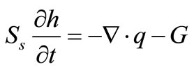 (3)
(3)
where Ss = specific storage q = flux h = Hydraulic head t = time The statement indicates that the change in hydraulic head with time equals the negative divergence of the flux (q) and the source (G).
Here the head and flux are unknown but Darcy’s law relates the flux to the head by substituting it in the flux, that is
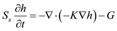 (4)
(4)
where G = external flow K = hydraulic conductivity Simplifying this we have
 (5)
(5)
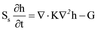
if K is replaced by it’s equivalent T, Equation (5) can be written as
 (6)
(6)
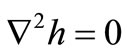
where: T = transmissivity A steady-state may be reached if the aquifer has recharging boundary conditions (or it may be used as an approximation in many cases). The equation describing this flow is a form of the Laplacian equation given as
 (7)
(7)
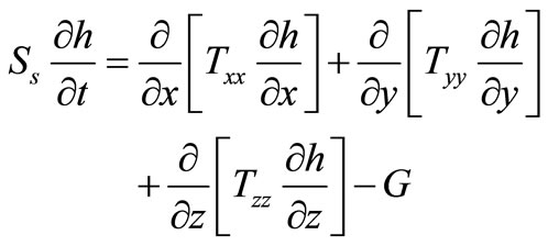
This equation states that hydraulic head is a harmonic function and has many analogs in other fields. The equation above can be rewritten as
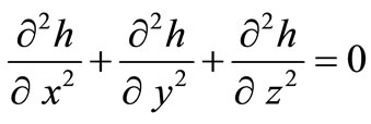 (8)
(8)
The above groundwater flow equations are valid for three dimensional flow.
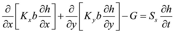
We also have two dimensional groundwater flow and the general governing equation is given by
 (9)
(9)
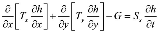
where k = hydraulic conductivity b = saturated thickness But, Kb = T, therefore:
 (10)
(10)
In finite difference form, eqn.10 can be expressed as:
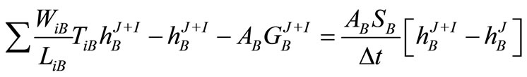 (11)
(11)
where Wi and Li are boundary width and flow path length.
A = Area of a single zone.
Groundwater velocity is based on hydraulic conductivity (k), as well as the hydraulic gradient (I). Therefore the equation determined by Darcy to describe the basic relationship between sub-surface material and the movement of water through them is
Q = KIA (12)
where Q = volumetric flow rate (Discharge)
K = Hydraulic conductivity
A = Area that the groundwater is flowing through
This relationship is known as Darcy’s law [11].
Rearranging Equation (12) we obtain the flux (V) which is known as the apparent velocity.
That is:
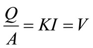 (13)
(13)
where V = Apparent velocity, m / sec The actual groundwater velocity which is called the Darcy’s flux (Vx) is given by
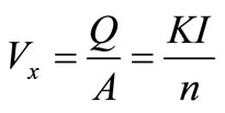 (14)
(14)
where Vx = Actual velocity m / sec n = Porosity This is the actual velocity of groundwater and does account for tortuosity of flow paths by including porosity in its calculation.
The Finite Difference Method is a computational procedure based on dividing an aquifer into a grid (see Figure 1) and analysing the flows associated within a single zone of the aquifer [12]. It utilizes a time distance grid of nodes and a truncated Taylor series approach to determine the condition of flow at any particular node. A brief coverage of the application of Taylor Series and nodal grid will illustrate several points fundamental to flow simulation.
The flow at time t, the profile of variable y with x may be described by a truncated Taylor Series given as
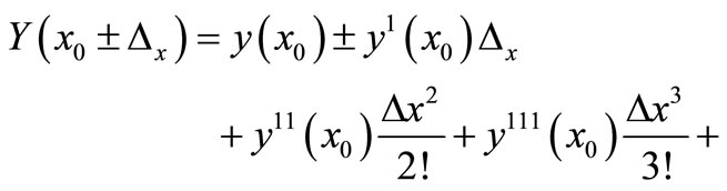 (15)
(15)
The value at x of node i is x0 and the + notation in equation 15 allows it to be used in forward or backward difference approach.
The forward difference first order is
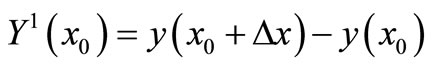 (16)
(16)
The backward difference first order is
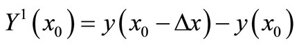 (17)
(17)
The summation of forward or backward difference also yields a central difference expression for the first order derivative of variable y at x0.
The central difference first order
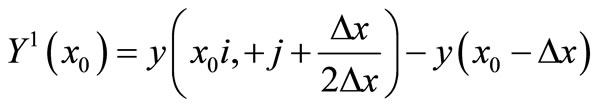 (18)
(18)
In computer notation, these equations (16-18) can be re-written as
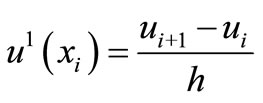
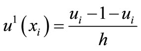
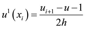
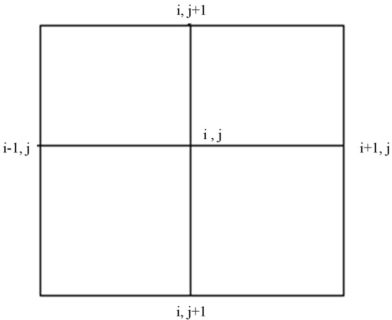
Figure 1. Computer notation for finite difference grid.
If there is recharge to the aquifer, a more useful result is the summation of the second order forward or backward difference forms of the truncated Taylor series to determine the second differential of variable y at x0 i.e.
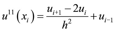 (19)
(19)
A special notation is used to describe the positions of the node in the finite difference grids.
In order to solve the groundwater flow equation we must be able to specify the initial and boundary conditions. There are two basic types of boundary conditions. If the head is known at the boundary of the flow region, this is known as a “Drichlet condition”. Then if the flux across a boundary to the flow region is known, this is known as “Neumann condition”. For a steady-state problem, boundary conditions are required; whereas for a transient problem, boundary and initial conditions must be specified. But in some cases the boundary conditions will be mixed with some portions having known head and some portions having known flux [13].Initial conditions and boundary conditions can be related to levels, pressure, and hydraulic head on the one hand (head conditions), or to groundwater inflow and outflow on the other hand (flow conditions).As an example of boundary conditions, let us consider Figure 2 below. This is a sand and gravel aquifer overlying an impermeable basement rock. There are several flow regions present, each leading away from a groundwater divide towards a stream. The plane of W to X is a groundwater divide. There is no flow across the divide and the boundary condition along the divide is
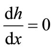 (20)
(20)
The plane of Z to Y is the centre of the stream and it is also a groundwater divide, across which no flow takes place. The boundary condition here is also:
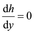 (21)
(21)
No flow occurs from the sand deposit into the impermeable bedrock, so along the X to Y plane there is no flow and the boundary condition is
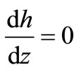 (22)
(22)
These three boundaries are Neumann boundaries where the flow conditions are specified.
2. Methods
A hypothetical site such as the one shown below (Figure 3) is chosen. The domain is discretized into an irregular
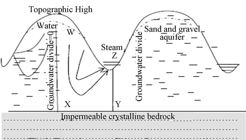
Figure 2. Boundary conditions for a cross section of a regional aquifer.
grid. Several different hydraulic heads and flux values are specified along the boundaries. A river enters the aquifer at the northern boundary and exits at the south. The production wells near the river withdraw water from the aquifer. Groundwater flow occurs mainly from the north to the south of the domain. The aquifer is hetero-
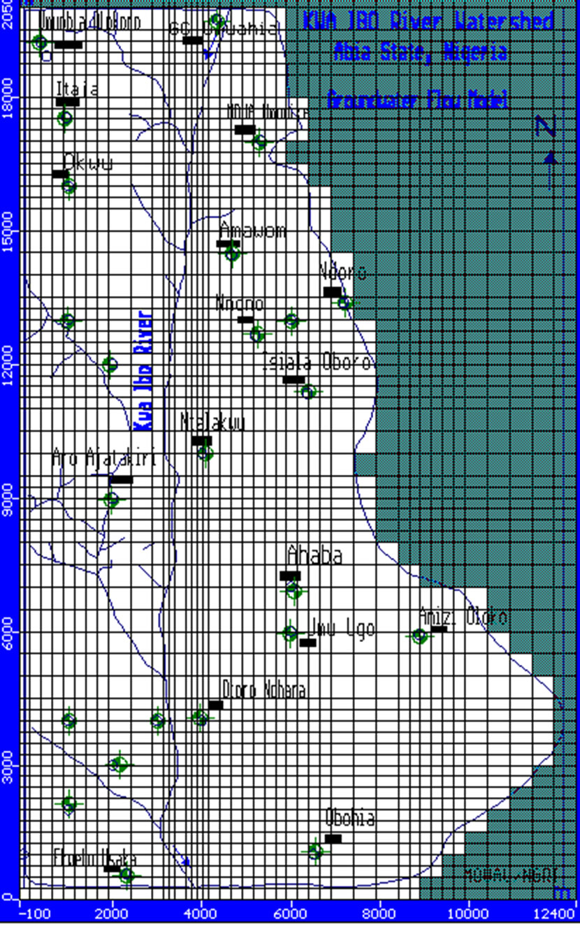
Figure 3. Discretized domain of a hypothetical site showing wells and river source.
geneous and anisotropic.
A finite difference grid is laid over an aquifer. It is a block centred finite difference grid where the node points fall in the centre of the grid. The grid parameters are:
Number of the grid columns 43
Number of grid rows 65
Minimum i coordinate 0
Minimum j coordinate 0
The basic grid is regular, with the rows and columns being normal to each other. The rows and columns may be varied so that there are more node points in certain parts of the aquifer than others. But this is desirable in the area around a well field.
For unconfined aquifers the saturated thickness bij is a function of the hydraulic heads. A priori both the hydraulic heads and the saturated thickness are unknown. Mathematically, this leads to non-linear behaviour. An initial guess for the saturated thickness is required in order to estimate the aquifer transmissivities Txxi,j and Tyyi,j. An iterative scheme must be used to calculate the hydraulic head distribution, update the transmissivities and check if the discrepancy between the previously estimated saturated thickness and the updated one is greater than a specific tolerance i.e.
New old
 > toleranc(23)
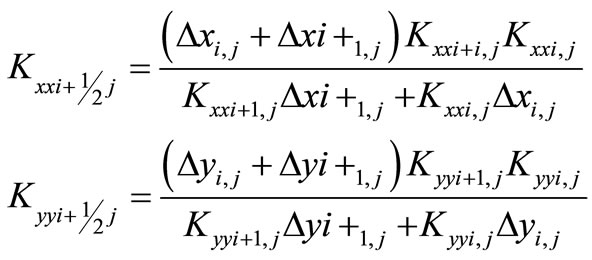
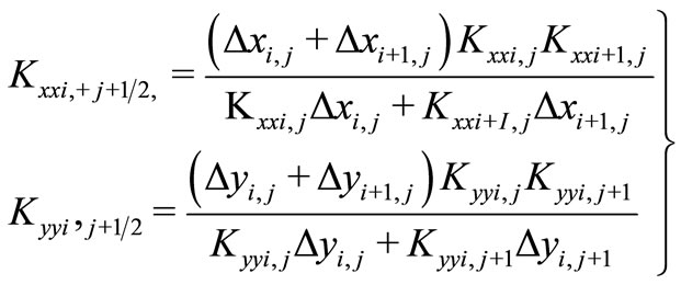
The directional transmissivities between adjacent nodes: Txxi + ½j, Tyyi, j + ½ are calculated by multiplying harmonic mean of hydraulic conductivities and geometric mean of saturated thickness [14].
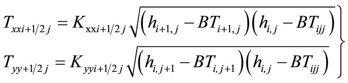 (24)
(24)
where BTi, j = aquifer bottom elevation at node i, j Kxxi + ½j, Kyyi + ½j = Hydraulic conductivities between blocks i, j and i+1, j .
 (25)
(25)
There are two different types of velocity vectors
(a) Nodal velocities
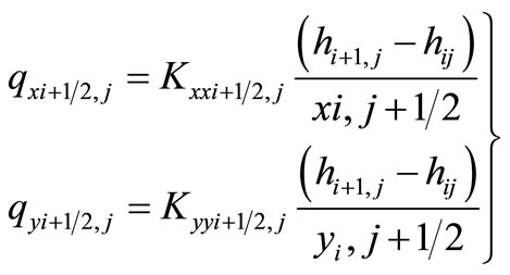
(b) Boundary velocities Boundary velocities are calculated directly from Darcy’s law using the hydraulic head difference and material properties between two nodes, whereas the nodal velocities are interpolated values at the grid nodes. The internodal components of the Darcy’s flux qx and qy are obtained by differentiation of the calculated hydraulic heads.
 (26)
(26)
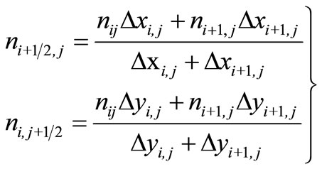
where, xi+ ½,j, yi,j + ½ = distance between nodes i, j and i +1, j and nodes i, j and i, j +1 respectively Kxxi + ½,j, Kyyi + ½, j = Hydraulic conductivities between i + i, j at x direction and nodes i, j and i, j +1 at y direction respectively These values are taken as the weighted harmonic mean between the hydraulic conductivities.
 (27)
(27)
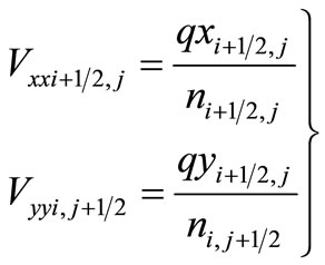
From the Darcy’s fluxes the pore velocities are calculated as:
 (28)
(28)
where ni + ½,j, ni,j + ½ = effective porosities between nodes i, j and i+1, j; and nodes i, j and i, j + 1 respectively. These values are taken as the weighted arithmetic mean between the porosities of adjacent blocks.
 (29)
(29)
Particle tracking provides a clearer description of groundwater flow within an aquifer. In steady-state flow field with no recharge, pathline (particle trace) coincides with streamlines. The two dimensional equation of pathlines is given by:
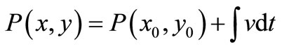 (30)
(30)
where P = Vector containing the x, y coordinates of the pathline.
P(xo,yo) = The starting point of the pathline (initial condition).
V = Average linear velocity t = Time Equation 30 is written in discretized form as an explicit time stepping scheme
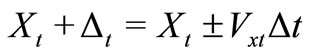
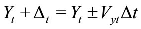
where
Δt = time increment, Vxt, Vyt, are the upstream components of the average linear velocity of the current particle locations at time t.
In this scheme, a set of uniformly distributed particles is assigned to each calculation cell. With each time step, every particle is moved to a new location based on velocity of the particle in the x and y directions. The velocity component at particle location is to be obtained from iterative scheme. In this scheme the particle representative area is assigned to each particle by dividing the cell into a set of equal number of squared sub cells with each particle at its centre.
The temporal weighted velocity is to be obtained by fourth order classical Runge Kutta method [15].
A weighted velocity is based on its values evaluated at four points in time, and then it is used to move the particle to a new direction.
Figure 4 shows the particle tracking algorithm. The aquifer is discretized using equally sized calculation cells. In the particle tracking scheme, one particle per cell is used.
3. Results and Discussion
The hydrodynamics of groundwater flow in a hypothetical aquifer chosen for this study has been found to depend mainly on the surface water flow within the site. The surface water flow is from north to south. So also is the groundwater. The aquifer is heterogeneous and anisotropic.
In the limiting case of a model calculation of an infinitely small grid space, the solution approaches the exact solution. Nodal and boundary velocities are calculated as the weighted harmonic mean between hydraulic conductivities and the arithmetic mean of the porosities of adjacent blocks. Initial and boundary conditions are used to specify the flow condition.
A numerical problem had been taken which allows the testing of numerical modelling technique called Finite Difference Method for the simulation of groundwater flow.
The region is bounded by two no flow boundaries as show in Figure 2. The aquifer is discretized using equally sized 2 x 2 calculation cells. In the scheme, one particle per cell is used.
Results from the flow chart of a particle tracking algorithm show that in a steady-state field with no recharge, pathlines coincide with streamlines. This means that the velocity component at particle location is obtained from iterative schemes.
It is also found that the accuracy of the numerical solution by Finite Difference Method is largely dependent on initial particle distribution and number of particles assigned to a cell. This scheme provides improved accuracy over interpolation scheme especially for block heterogeneous aquifer but with increased computational efforts.
4. Conclusions
Numerical modelling has found interesting application in groundwater flow and transport since the mid-1960 s, when digital computers with adequate capacity became generally available. The need for a numerical model cannot be over emphasized since analytical models assume a homogenous aquifer.
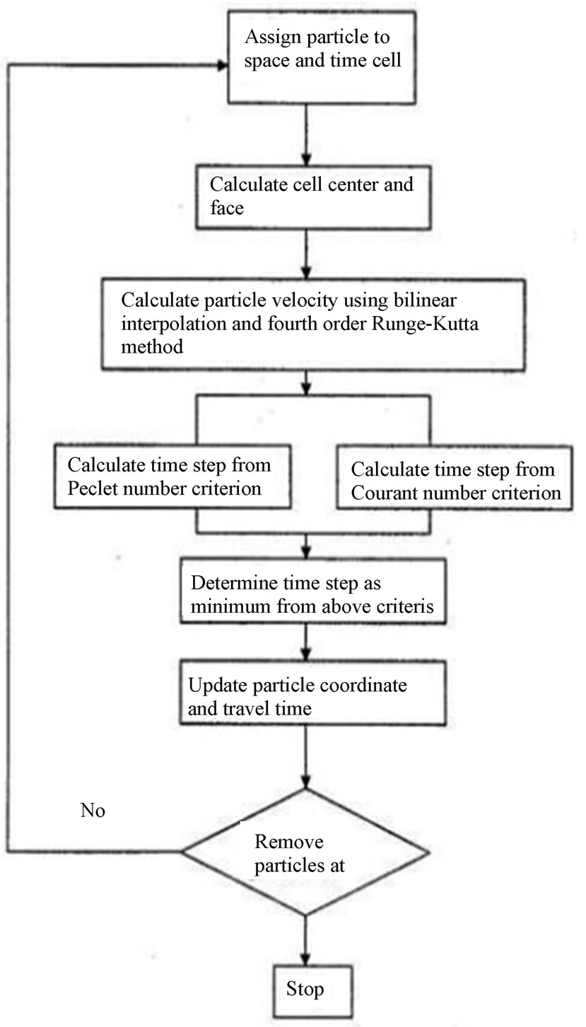
Figure 4. Flowchart of the computational algorithm for particle tracking.
The numerical method applied in this study is the Finite Difference Method, which in its simplicity provides necessary aids in finding solution to groundwater problems.
The finite difference grid overlain over the aquifer improves the accuracy in the calculation of flow rate and direction. It is also an advantage in particle tracking within the aquifer domain. The modelling studies have been carried out in a hypothetical site with the aim of determining rate and direction of flow of groundwater through an aquifer domain. The domain is discretized with boundary conditions considered for easy calculations.
In the flow model it was observed that water flows from region of high hydraulic head to region of low hydraulic head and that an exact solution could be obtained if the grid spacing is small enough say 5 cm. Results show that in a steady-state flow field with no recharge, pathlines coincide with streamlines. It is therefore concluded that Finite Difference Method can be used to predict the future direction of flow and particle location within a simulation domain.
REFERENCES
- R. A. Freeze, “Three Dimensional Transient Saturated– Unsaturated Flow in a Groundwater Basin,” Water resources Research, 1979, pp. 347-366.
- L. F. Konikow and J. D. Bredehoeft, “Computer Model of Two Dimensional Solute Transport and Dispersion in Groundwater,” U.S. Geological Survey, Techniques of Water Resources Investigation Book 7, Chapter C2, 1992, p. 90.
- V. Vu.Hung and Ramin S. Estandiari, “Dynamic Systems: Modelling and Analysis,” McGraw-Hill, New York, 1997 p. 612.
- J. M. McDonald and A. W. Harbaugh, “A Modular Three-Dimensional Finite-Difference Groundwater Flow Mode,” Techniques of Water Resources Investigations of the U. S. Geological Survey Book.6, 1988, p. 586.
- T. Narasimha Reddy and V. V. S. Gurunadha Rao, “water Balance Model and Groundwater Flow Model of Dulapally Basin,” Granitic Terrain, A.P., Research Series No. 9, 1991.
- M. P. Anderson and W. W. Woessner, “Applied Groundwater Modeling, Simulation of Flow and Advective Transport,” Academic Press, San Diego, C. A, 1992.
- M. U. Igboekwe, V. V. S. Gurunadha Rao and E. E. Okwueze, “Groundwater Flow Modelling of Kwa Ibo River Watershed Southeastern Nigeria,” Hydrological Processes, Vol. 22, No. 10, 2008, pp. 1523-1531. doi:10.1002/hyp.6530
- M. K. Hubbert, “Darcy’s Law and Field Equations of Flow of Underground Fluids Transaction,” American Institute of Mining and Metallurgical engineers, 1956, pp. 22-239.
- T. A. Prickette and C. G. Longuist, “Selected Digital Computer Techniques for Groundwater Resource Evaluation,” Bull.55, Illinois State Water Survey, Urbana, 1981. p. 62.
- W. J. Gray and J. L. Hoffman, “A Numerical Model Study of Ground-Water Contamination from Price's Landfill, New Jersey — I. Data Base and Flow Simulation,” Groundwater, Vol. 21, No. 1, 1983, pp. 7-14. doi:10.1111/j.1745-6584.1983.tb00699.x
- D. K. Todd, “Groundwater Hydrology,” 2nd Edition, John Wiley and Sons, New York, 2001.
- Peter. C. Trescott and S. P. Larson, “Finite Difference Model for Aquifer Simulation in Two-Dimensions with Results of Numerical Experiments,” U.S. Geological Survey Techniques at Water-Resources Investigations, Book 7, Chapter C1, 1976, p. 116.
- C. W. Fetter, “Applied Hydrogeology: Finite Difference Model,” CBS Publishers and Distributors, New Delhi, India, 2000, p. 592.
- M. U. Igboekwe, “Geoelectrical Exploration for GroundWater Potentials in Abia State, Nigeria,” An Unpublished PhD dissertation. Michael Okpara University of Agriculture, Umudike, 2005, p. 131.
- R. T. Peter, “Numerical Analysis: Runger–Kutta Method,” ISBN 0. 333 -58665- 4, 1994, pp. 214-217.