Journal of Water Resource and Protection
Vol. 3 No. 1 (2011) , Article ID: 3780 , 9 pages DOI:10.4236/jwarp.2011.31008
Spectral Geometric Triangle Properties of Chlorophyll-A Inversion in Taihu Lake Based on TM Data
1The Key Laboratory of Marine Hydrocarbon Resources and Environmental Geology, Qingdao, China
2Qingdao Institute of Marine Geology, Qingdao, China
3College of Resources Sciences and Technology, Beijing Normal University, Beijing, China
E-mail: cjun@cgs.cn
Received October 24, 2010; revised November 28, 2010; accepted December 27, 2010
Keywords: Water Quality, Remote Sensing, Invsersion Model, Chlorophyll-a Concentration, Taihu Lake
ABSTRACT
The main objective of this study was to develop and validate the applicability of the Area Chlorophyll-a Concentration Retrieved Model (ACCRM), Height Chlorophyll-a Concentration Retrieved Model (HCCRM), Angle Chlorophyll-a Concentration Retrieved Model (AgCCRM), and Ratio Model of TM2/TM3 (RM) in estimating the chlorophyll-a concentration in Case = 2 \* ROMAN II water bodies, such as Taihu Lake in Jiangsu Province, China. Water samples were collected from 23 stations on the 27th and 28th of October, 2003. The four empirical models were calibrated against the calibration dataset (samples from 19 stations) and validated using the validation dataset (samples from 4 stations). The regression analysis showed higher correlation coefficients for the ACCRM and the HCCRM than for the AgCCRM and the Ratio Model; and the HCCRM was slightly superior to the ACCRM. The performance of the ACCRM and the HCCRM was validated, and the ACCRM underestimated concentration values more than the HCCRM. The distribution of chlorophyll-a concentrations in Taihu Lake on October 27, 2003 was estimated based on the Landsat/TM data using the ACCRM and the HCCRM. Both models indicated higher chlorophyll-a concentrations in the east, north and center of the lake, but lower concentrations in the south. The accuracy of results obtained from the HCCRM and the ACCRM were also supported by the validation dataset. The study revealed that the HCCRM and the ACCRM had the best potential for accurately assessing the chlorophyll-a concentration in the highly turbid water bodies.
1. Introduction
In recent years, many coastal and inland waters have become enriched with nutrients and now support excessive increases in the chlorophyll-a concentration [1]. Remote sensing technology has been proposed as a useful means to improve the capability of estimating the chlorophyll-a concentration accurately [2-4]. It is well known that the water optical properties can provide quantitative information on the optically significant materials presented in water bodies. The bands ranging from 400 nm to 750 nm are most commonly used to estimate the chlorophyll-a concentration [5-9].
A variety of algorithms have been developed for estimating the chlorophyll-a concentration in Case I water, including empirical and semi-analytical models [7,10,11]. Most of these algorithms were based on the spectral properties near the region of 700 nm. Another widely applied parameter was the ratio of the near-infrared peak reflectance to the reflectance around 675 nm, which represents the red absorption peak of the chlorophyll-a [12]. For example, Gons et al. [13] first derived the backscattering coefficient at 704 nm and 672 nm, and then used the reflectance and absorption at these two wavelengths to predict the chlorophyll-a concentration; and Tiemann & Kaufman [14] used the ratio of 705 nm to 678 nm to estimate the chlorophyll-a concentration in the Mecklenburg Lake. More complex relationships have also been suggested. Gitelson et al. [15] developed the three-band model for MERIS spectral bands to estimate the chlorophyll-a concentration in turbid waters. Le et al. [12] used an improved algorithm of three-band and four-band models to assess the chlorophyll-a concentration in Taihu Lake.
The most widely applied models used for the chlorophyll-a concentration estimation assume that the optical parameters, such as the chlorophyll-a and the specific absorption coefficient, are constant. This assumption considerably impacts their accuracy [16-18], especially in the turbid water bodies like Taihu Lake. Additionally, most applied models are not suitable for multi-band remote sensors, such as the Landsat/TM, which prohibits their use with widely-available remote sensing resources. In this study, empirical models are introduced for the chlorophyll-a concentration retrieval based on the TM data for the turbid waters of Taihu Lake in China. The primary goal of this paper was to develop and validate these models and to determine their suitability for estimating the chlorophyll-a concentration distribution in Taihu Lake on October 27, 2003.
2. Materials and Methods
2.1. Data Acquisition
Located in east China, the Taihu Lake (Figure 1(a)) is a typical inland water body, influenced by river and human activity inputs with a low deposition rate. Because the water is highly turbid, the Taihu Lake was selected for this study. It was difficult to estimate the chlorophyll-a concentration of this lake accurately, as the optical properties of the water show great spatiotemporal variability [19]. The absorption signal of the chlorophyll-a from phytoplankton is partly overwhelmed by that of the suspended solids and backscattering. As a result, it is difficult to estimate the chlorophyll-a concentration accurately using conventional methods, such as the multiple bands and single band algorithms.
In situ measurements were carried out in the Taihu Lake on the 27th and 28th of October, 2003, which coincided with acquisition of Landsat-5/TM imagery for the lake. During the period of the satellite overpass (about ±1h) on October 27, 2003, the in situ measurements were carried out with the ASD field spectrometer at each station. Therefore, it is reasonable to assume that the in situ experiment on the ground was approximately synchronized with the satellite observation from space. The distribution of in situ sampling points is depicted in Figure 1(a) and the spectral curves of the in situ measurements are shown in Figure 1(b). The reflectance measurements were performed using a spectroradiometer with 25° fore-optic, covering the 350 nm-2500 nm spectral domain (Analytic Spectral Devices (ASD), Boulder, CO). The ASD had a spectral resolution of 3 nm (full-width-at-half-maximum, FWHM) and a 1.4nm sampling interval across the 350 nm-1050 nm spectral range [20]. The resulting data were interpolated by the ASD software during the collection to produce values at 1nm intervals. The experiments were conducted strictly in compliance with the Ocean Optical Protocols of NASA [21]. In order to compute the sub-surface irradiance reflectance, the radiance was measured from a calibrated reflectance panel before and after shading. Hyperspectral reflectance was calculated as follows [21]:
 (1)
(1)
where  is the water-leaving radiance,
  is the total incident radiant flux of the water surface, and
  is the remotely sensed reflectance.
  and
and  in
in
 (a)
(a)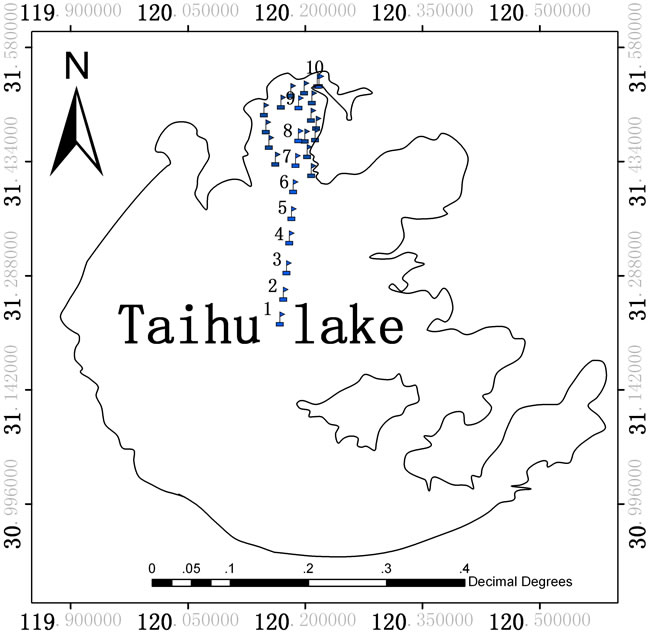 (b)
(b)
Figure 1. The Taihu lake. (a) The location of the Taihu lake, with the blue flags representing the distributions of the in situ measurements; (b) in situ measurements of spectral curves corresponding to the sampling points in figure 1(a).
Equation (1) are further calculated as follows [12]:
 (2)
(2)
 (3)
(3)
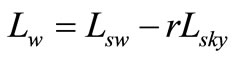
where  denotes the total radiance received from the water surface;
  represents the diffused radiation of the sky, which contains no information on water properties, and hence has to be eliminated; r refers to the reflectance of the skylight at the air-water interface, whose value depends upon the solar azimuth, measurement geometry, wind speed, and surface roughness;
  is the radiance of the gray board; and
  is the reflectance of the gray board, which is accurately calibrated to 30%.
The limnological sampling was performed on the same day using a rosette sampler or bucket. After sampling, bottles with water samples were maintained at a low temperature and sent for laboratory analysis in the same day they were collected.
The in situ water sample measurements were divided randomly into two sets. One set was used to calculate the parameters of retrieving models, and included the dataset of 19 stations (called the “calibration data” below). The other set was used to validate the accuracy of the retrieving models, and included the dataset of 4 stations (called the “validation data” below).
2.2. Reflectance Calibration
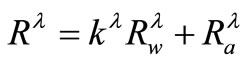
Among the total signals received by the sensor at satellite altitudes, over 80% of that typically in blue spectral region was from the contribution of light scattering by molecules and aerosol particles in the atmosphere [22,23]. Thus, the water-leaving radiance, from which the phytoplankton concentration was derived, was only a portion of the total radiance arriving at the sensor. The process of retrieving the water-leaving radiance from the total radiance is usually referred to as the atmospheric correction. The general atmospheric correction algorithm was adopted to make an assessment of the corresponding band reflectance of imagery by using the special near-infrared spectral bands, whose reflectance is supposed to be zero in Morel’s Case I waters [22-24]. However, this standard atmospheric correction method is not applicable to the turbid water bodies, such as Taihu Lake, owing to the scattering at this wavelength by detrital material. Additionally, the near-infrared data from TM4 has been shown to exhibit an almost linear relationship with increasing quantities of suspended matter [17]. As a result, the atmospheric correction developed for clear water bodies by Gordon & Clark [24] is not applicable to the Case II water bodies [22,24].
In addition to the atmospheric effects, the adjacency effects are also highly significant in data acquired by the high spatial resolution sensors, such as the Landsat/TM [25]. Ouaidrari & Vermote [26] showed that the adjacency effects were strongly linearly related with the surface reflectance of imagery pixels. In order to eliminate the sensors sensitivity to atmospheric influences and adjacency effects, the water-leaving reflectance ( ) from in situ measurements were used in this study to calibrate the reflectance (
 ) of the Landsat/TM imagery by Line Empirical Model for Reflectance Calibration (LEMRC) [27-29] as follows:
 (4)
(4)
where  is the wavelength,
  is the attenuation coefficient corresponding to the wavelength
 ;
;  is the atmospheric contributions to the reflectance; and
  and
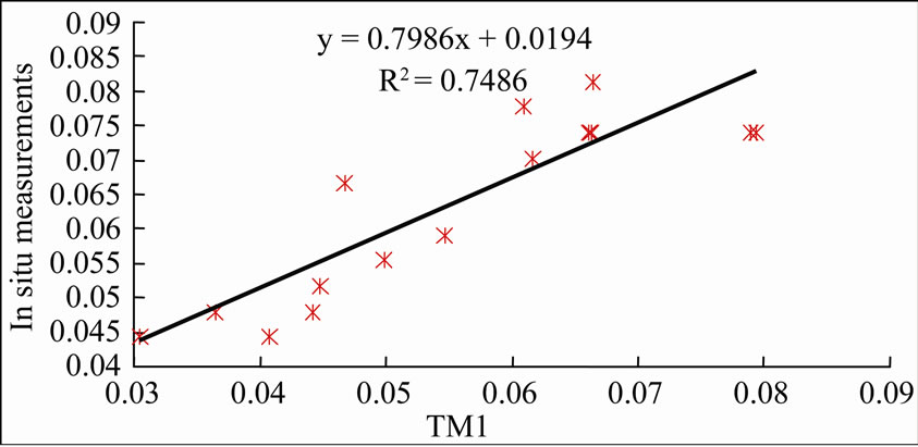
and  are considered as constants at a given wavelength and are approximated using the regression shown in Figure 2.
2.3. Constructions of Four Empirical Models
Various constituents of environmental water samples, such as the phytoplankton cells, detrital material, and colored dissolved organic matter (CDOM), affected the passage of light through the sample by scattering and absorption In general, the reflectance at lower wavelengths of 400-500 nm was relatively low due to the combined affects of absorption by the CDOM, tripton and phytoplankton pigments. A local maximum in reflectance around 550 nm-580 nm was caused by a local minimum in the combined effects of the low phytoplankton pigment absorption efficiency and lower CDOM and tripton absorption. A clear reflectance minimum was located at 676 nm, which corresponds to the in vivo chlorophyll-a maximum absorption peak. Beyond 680 nm, the reflectance increased significantly and reached a maximum at 706 nm [17]. This maximum could be used for interpretation of the signal due to the natural phytoplankton fluorescence [30], however, the Landsat/TM data did not have bands in this area.
The spectral absorption features, such as the height, area, and angle (Figure 3), have been widely used in the vegetation canopy remote sensing field studies. Shrestha et al. [31] used the absorption width, area and depth of reflectance curves for mapping land degradation. Walsh et al. [32] applied the Hyperion data and QuickBird data for the control and management of land use based on the analysis of those spectral characteristics due to an invasive plant species. This study explores the geometric triangle properties of multiple spectral remote sensing data to retrieve the chlorophyll-a concentration.
 (a)
(a)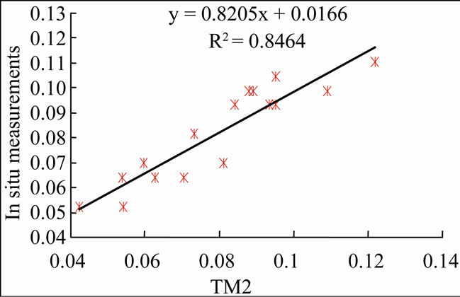 (b)
(b) (c)
(c)
Figure 2. Relationships between the reflectance of TM imagery and in situ measurements at TM1, TM2 and TM3, respectively.
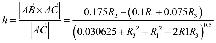
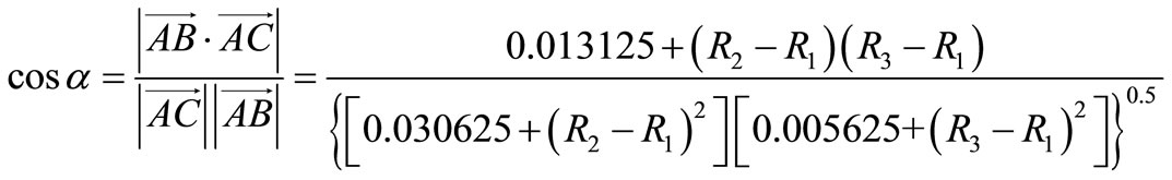
As shown in Figure 3, the lines AB, BC and AC denoting the vectors were as follows:
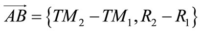 (5)
(5)
 (6)
(6)
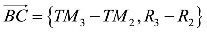 (7)
(7)
The area of triangle ABC, S, was calculated as follows:
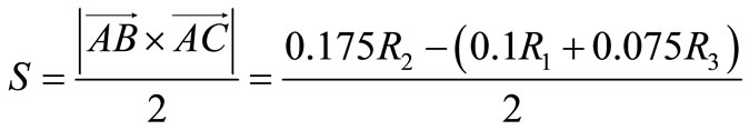 (8)
(8)
The high of triangle ABC, h, was calculated as follows:
 (9)
(9)
One angle of triangle ABC, α, was calculated as follows:
The spectral curves in Figure 1(b) show that the reflectance in the blue region (400-500 nm) was relatively low owing to high absorption by components of the water samples. The reflectances in the green region (500-600 nm) and red region (600-700 nm) were the primary and the secondary reflectance peaks, respectively, and result from the scattering of the suspended sediments and low absorption coefficients of both CDOM and chlorophyll-a pigment. Additionally, the reflectance in the blue region of the visible spectrum decreased at a rate nearly equivalent to that of the reflectance elevation in the green and red regions [33]. Due to the differential reflectance of the phytoplankton pigments at different wavelengths, the shape of the triangle as shown in Figure 3 would be deformed, resulting in the variance of the height, the area and the angle of the triangle. Accordingly, it was indicated that the geometrical quantities, such as the angle, height and area were strongly correlated with the reflectance at the three visible bands of the Landsat/TM image. According to these properties and a combination of Equation (8), Equation (9) and Equation (10), the geometrical quantities, such as the angle, height and area, were found to correlate excellently with the chlorophyll-a concentration.
3. Results and Discussion
3.1. Empirical Models
3.1.1. Model Calibration
To match the bandwidth of Landsat/TM, the ASD measurements were aggregated using the Landsat/TM sensor
 (10)
(10)
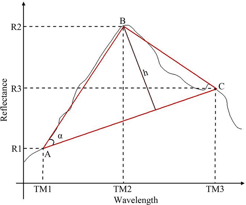
Figure 3. The triangle properties between the three visible bands of Landsat; R1, R2 and R3 represent the remote sensing reflectance at TM1, TM2 and TM3; h represents the height of the triangle when the baseline is AC; α is the angle of < BAC.
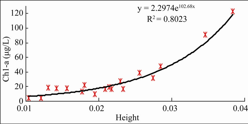
spectral response functions before model calibration. The Landsat/TM sensor spectral response functions used in this study were suggested by Vries et al. [34]. All of these common empirical models were tested to determine the relationship between the chlorophyll-a concentration and the triangular geometric quantitative parameters. The geometrical variables of height and area were exponentially well correlated with the chlorophyll-a concentration in Taihu Lake (Figure 4). The regression coefficients of the HCCRM and ACCRM were 0.8023 and 0.7985, respectively. The regression coefficients of the HCCRM and ACCRM were higher than that of the RM, which was 0.3124. Interestingly, the relationship between the chlorophyll-a concentration and the geometrical variable of angle was not ideal. The correlation coefficient of the AgCCRM was only 0.001.
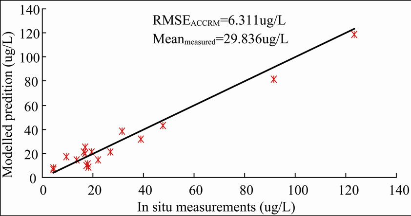
Figure 5 illustrates the relationship between the modeled prediction of HCCRM and ACCRM and the calibration data. Compared with the RM. both algorithms appeared perfectly suitable for estimating the chlorophyll-a concentration, though the ACCRM had a slightly superior performance compared with the HCCRM. Using HCCRM to estimate the chlorophyll-a concentration in Taihu Lake reduced the correlation coefficient of 0.0038 from HCCRM, and the Root Mean Square Error (RMSE) was decreased from 6.311 mg/L for ACCRM to 6.273 mg/L for HCCRM, while the mean measured value of the chlorophyll-a concentration of calibration data was 29.836 mg/L.
The relationship between the predicted chlorophyll-a concentration and the calibration data also revealed the ability of the two approaches in retrieving the chloro-
 (a)
(a)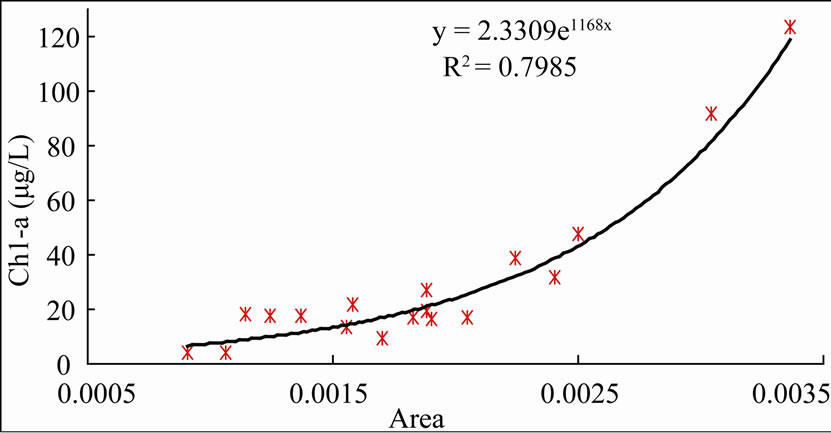 (b)
(b)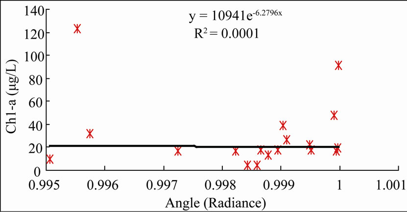 (c)
(c)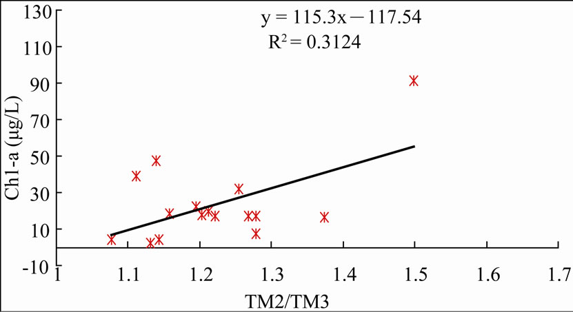 (d)
(d)
Figure 4. Empirical models. (a), (b) and (c) represent the linear empirical model based on the height, area and angle of triangle ABC, respectively; (d) represents the linear model based on the band ratio of TM2 to TM3.
phyll-a concentration. Figure 5 shows a plot of predicted chlorophyll-a concentrations versus in situ measured
 (a)ACCRM
 (b)HCCRM
Figure 5. Assessment of retrieval results. (a) presents the relationship between the chlorophyll-a concentration predictions of ACCRM and calibration data; (b) presents the relationship between the chlorophyll-a concentration predictions of HCCRM and calibration data.
values. Almost all points converged along the line of  (where,
  denotes the in situ measured chlorophyll-a concentrations and
  denotes the chlorophyll-a concentrations predicted by the model). Despite minor differences in relative correlation coefficients and RMSE, the HCCRM and ACCRM were both suitable for chlorophyll-a concentration estimation in Taihu Lake. An additional operator of
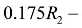
 was included in the HCCRM and ACCRM. The coefficient value before term of
  equals the sum of the coefficients before the terms of
  and
and , but the signs are opposite. This operator allows the model to eliminate some atmospheric influences, such as the linear effects on the bands of TM1, TM2, and TM3, which theoretically improves the accuracy of the retrieved results.
3.1.2. Model Validation
The performance of the HCCRM and ACCRM was evaluated by examining their respective RMSE in estimating the chlorophyll-a concentration. Figure 6 shows the relationship between the modeled prediction of HCCRM and ACCRM and the validation data. Both models produced accurate chlorophyll-a concentration predictions, but the performance of the HCCRM was slightly superior to that of the ACCRM. Compared with ACCRM, the uncertainty in estimating the chlorophyll-a concentration in Taihu Lake decreased by 2.39% with the use of the HCCRM, and the RMSE also decreased from 4.276 mg/L in ACCRM to 3.858 mg/L in HCCRM. The regression coefficient was 0.8023 in HCCRM and 0.7985 in ACCRM. The performances of HCCRM and ACCRM using the calibration data were consistent with those using the validation data. Additionally, the total errors between the modeled prediction and the validation data were used to estimate the total bias of the retrieved results. According to Figure 6, the total bias was –4.003 mg/L in ACCRM and –3.570 mg/L in HCCRM. Therefore, it was concluded that the HCCRM and ACCRM were both suitable for detecting and mapping the chlorophyll-a concentration in Taihu Lake on October 27, 2003, yet the HCCRM was slightly more accurate than the ACCRM.
3.2. Chlorophyll-A Mapping Based on TM Data
To estimate the water-leaving radiance from the total radiance measured at the sensor, the LEMRC (Figure 2) was used as the atmospheric correction algorithm to eliminate the atmospheric influence of TM1, TM2 and TM3 of Landsat images. Then the HCCRM and ACCRM were used to map the chlorophyll-a concentration in Taihu Lake.
Figure 7(a) and Figure 7(b) shows the chlorophyll-a maps of Taihu Lake on October 27, 2003 calculated from the HCCRM (Figure 4(a)) and ACCRM (Figure 4(b)), respectively. Overall, the chlorophyll-a concentrations throughout Taihu Lake, calculated by either HCCRM or ACCRM, were higher in the east, north and center of the lake but lower in the south of the lake (Figure 7). However, some significant differences could be found between the results from the two algorithms. The concentration range was 0-100 mg/L in HCCRM and 0-130 mg/L in ACCRM. The concentrations estimated by
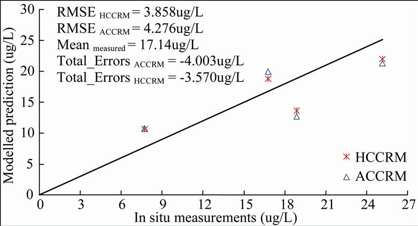
Figure 6. Relationship between the modeled prediction of HCCRM and ACCRM and validation data.
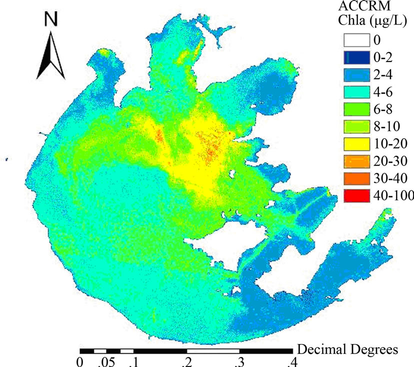 (a) Chlorophyll-a map estimated by ACCRM
 (b) Chlorophyll-a map estimated by HCCRM
 Figure 7. Inversion results of the exponential empirical model of ACCRM and HCCRM as shown in Figure 3(a).
ACCRM were higher than those by HCCRM, especially at the prominent concentration range of 6-10 mg/L. The total biases of HCCRM and ACCRM given in Figure 6 reveal that the chlorophyll-a concentrations predicted by ACCRM were more underestimated than those by HCCRM.
4. Conclusions
Empirical algorithms are easy and straightforward for data processing. However, because the empirical coefficients contained in the empirical algorithms are derived from the data set they may not necessarily account for all natural variations. In this study, four experimental models for estimating the chlorophyll-a were constructed by specifying the remotely sensed parameters. They are the area, the height, the angle of a triangle and band ratio of TM2 to TM3. Using the calibration dataset, the evaluation of samples collected in Taihu Lake, China, on the 27th and the 28th of October, 2003, ACCRM and HCCRM showed better performance than the band ratio algorithms and AgCCRM. The HCCRM was slightly superior to the ACCRM based on the correlation coefficient and RMSE.
The performance of ACCRM and HCCRM was validated by the validation dataset. Both algorithms underestimated the chlorophyll-a concentration in Taihu Lake on October 27, 2003. The total bias was –4.003 mg/L in ACCRM and –3.570 mg/L in HCCRM, so the ACCRM underestimated more than the HCCRM. As a whole, both algorithms showed the spatial distribution of chlorophyll-a concentration was higher in the east, north and center of the lake, but was lower in the south of the lake. The concentration estimated by ACCRM was higher than that by HCCRM, especially at the prominent concentration range of 6-10 mg/L.
5. Acknowledgement
This study was supported by the National Key Technology R & D Program in the 11th Five Year Plan of China (2008BAC34B03) and the China National Great Geological Survey (GZH200900504).
REFERENCES
- D. G. George, “The Airborne Remote Sensing of Phytoplankton Chlorophyll-A in the Lakes and Tarns of the English Lake District,” International Journal of Remote Sensing, Vol. 18, No. 9, 1997, pp. 1961-1975. doi:10.1080/014311697217972
- P. A. Tester and R. P. Stumpf, “Phytoplankton Blooms and Remote Sensing: What is the Potential for Early Warning,” Journal of Shellfish Resources, Vol. 17, No. 5, 1998, pp. 1469-1471.
- J. B. Michael and B. Emmanuel, “The Beam Attenuation to Chlorophyll-A Ratio: An Optical Index of Phytoplankton Physiology in the Surface Ocean,” Deep-Sea Research, Vol. 50, 2003, pp. 1537-1549.
- L. H. Kantha, “A General Ecosystem Model of for Applications to Primary Productivity and Carbon Cycle Studies in the Global Oceans,” Ocean Modeling, Vol. 6, No. 3-4, 2004, pp. 285-334. doi:10.1016/S1463-5003(03)00022-2
- A. Morel and L. Prieur, “Analysis of Variances in Ocean Color,” Limnology and Oceanography, Vol. 22, 1977, pp. 709-722. doi:10.4319/lo.1977.22.4.0709
- H. R. Gordon and A. Y. Morel. “Remote Assessment Ocean for Color Interpretation of Satellite Visible Imagery,” 1st Edition, New York, Springer Verlag, England, 1983, pp. 31-107.
- C. D. Mobley, “Light and Water: Radiative Transfer in Natural Waters,” 1st Edition, Academic Press, London, England, 1994, pp. 21-69.
- S. Tassan, “A Numerical Model for the Detection of Sediment Concentration in Stratified River Plumes Using Thematic Mapper Data,” Internal Journal of Remote Sensing, Vol. 18, No. 12, 1997, pp. 2699-2705. doi:10.1080/014311697217567
- P. Chauhan, M. Mohan, R. K. Sarngi, B. Kumari and S. G. P. Matondkar, “Surface Chlorophyll-A Estimation in the Arabian Sea Using IRS-P4 Ocean Colour Monitor (OCM) Satellite Data,” Internal Journal of Remote Sensing, Vol. 23, No. 8, 2002, pp. 1663-1676. doi:10.1080/01431160110075866
- H. R. Gordon, O. B. Brown, R. H. Evans, J. W. Brown, R. C. Smith, K. S. Baker and D. K. Clark. “A Semi-Analytic Radiance Model of Ocean Color,” Journal of Geophysical Research, Vol. 93, No. D9, 1988, pp. 10909-10924. doi:10.1029/JD093iD09p10909
- I. Joint and S. B. Groom, “Estimation of Phytoplankton Production from Space: Current Status and Future Potential of Satellite Remote Sensing,” Journal of Experimental Marine Biology and Ecology, Vol. 250, No. 1, 2000, pp. 233-255. doi:10.1016/S0022-0981(00)00199-4
- C. F. Le, Y. M. Li, Y. Zha, D. Y. Sun, C. C. Huang and H. Lu, “A Four-Band Semi-Analytical Model for Estimating Chlorophyll-A in Highly Turbid Lakes: The Case of Taihu Lake, China,” Remote Sensing of Environment, Vol. 113, No. 6, 2009, pp. 1175-1182. doi:10.1016/j.rse.2009.02.005
- H. J. Gons, M. Rijkeboer, S. Bagheri and K. G. Ruddick, “Optical Teledetection of Chlorophyll-A in Estuarine and Coastal Waters,” Environmental Science and Technology, Vol. 34, No. 24, 2000, pp. 5189-5192. doi:10.1021/es0012669
- S. Tiemann and H. Kaufman, “Determination of Chlorophyll-A Contentand Tropic State of Lakes Using Field Spectralmeter and IRS-IC Satellite Data in Mecklenburg Lake Distract, Germany,” Remote Sensing of Environment, Vol. 73, No. 2, 2000, pp. 227-235.
- A. A. Gitelson, G. D. Olmo, W. Moses, D. C. Rundquist, T. Barrow, T. R. Fisher, D. Gurlin and J. Holz, “A Simple Semi-Analytical Model for Remote Estimation of Chlorophyll-A in Turbid Waters; Validation,” Remote Sensing of Environment, Vol. 112, No. 9, 2008, pp. 3582-3593. doi:10.1016/j.rse.2008.04.015
- G. K. Yew-Hoong, S. T. Koh, I. I. Lin and E. S. Chan, “Application of Spectral Signatures and Colour Ratios to Estimate Chlorophyll-A in Singapore’S Coastal Waters,” Journal of Photogrammetry and Remote Sensing, Vol. 55, 2001, pp. 719-748.
- A. G. Dekker, R. J. Vos and S. W. M. Peters, “Analytical Algorithms for Lake Water TSM Estimation for Retrospective Analysis of TM and SPOT Sensor Data,” International Journal of Remote Sensing, Vol. 23, No. 1, 2002, pp. 15-35. doi:10.1080/01431160010006917
- G. Dall’Olmo and A. A. Gitelson, “Effect of Bio-Optical Parameter Variability and Uncertainties in Reflectance Measurements on the Remote Sensing Estimation Of Chlorophyll-A Concentration in Turbid Productive Waters: Modeling Results,” Applied Optics, Vol. 45, No. 15, 2006, pp. 3577-3592. doi:10.1364/AO.45.003577
- Y. L. Zhang, B. Zhang, X. L. Wang, S. Feng and Q. H. Zhao, “A Study of Absorption Characteristics of Chromophoric Dissolved Organic Matter and Particles in Lake Taihu, China,” Hydrobiologia, Vol. 592, 2007, pp. 105- 120. doi:10.1007/s10750-007-0724-4
- ASD, “Analytic Spectral Devices, Inc. Technical Guide,” 3rd Edition, Boulder, Colorado, 1999.
- J. L. Mueller and R. W. Austin, “Ocean Optics Protocols for Seawifs Validation,” NASA Techmical Memorandum 104566, Greenbelt, MD, NASA Goddard Space Flight Center, 1992.
- K. Y. Ding and H. R. Gordon, “Atmospheric Correction of Ocean-Color Sensors: Effects of the Earth’S Curvature,” Applied Optics, Vol. 33, No. 30, 1994, pp. 7096- 7106. doi:10.1364/AO.33.007096
- H. R. Gordon and M. H. Wang, “Retrieval of WaterLeaving Radiance and Aerosol Optical Thickness over the Oceans with Seawifs: A Preliminary Algorithm,” Applied Optics, Vol. 33, No. 3, 1994, pp. 443-452. doi:10.1364/AO.33.000443
- H. R. Gordon and D. K. Clark, “Clear Water Radiances for Atmospheric Correction of Coastal Zone Color Scanner Imagery,” Applied Optics, Vol. 20, No. 24, 1981, pp. 4175-4180. doi:10.1364/AO.20.004175
- M. Putsay, “A Simple Atmospheric Correction Method for the Short Wave Satellite Image,” International Journal of Remote Sensing, Vol. 13, No. 8, 1992, pp. 1549- 1558. doi:10.1080/01431169208904208
- H. Ouaidrari and E. F. Vernote, “Operational Atmospheric Correction of Landsat TM Data,” Remote Sensing of Environment, Vol. 70, 1999, pp. 4-15. doi:10.1016/S0034-4257(99)00054-1
- J. R. Apel, “An Improved Model of the Ocean Surface Wave Vector Spectrum and Its Effects on Radar Backscatter,” Journal of Geophysical Research, Vol. 99, No. C8, 1994, pp. 16269-16291. doi:10.1029/94JC00846
- W. H. Farrand, R. B. Singer and E. Merenyi, “Retrieval of Apparent Surface Reflectance from AVIRIS Data: A Comparison of Empirical Line, Radiative Transfer, and Spectral Mixture Methods,” Remote Sensing of Environment, Vol. 47, No. 3, 1994, pp. 311-321. doi:10.1016/0034-4257(94)90099-X
- G. Ferrier, “Evaluation of Apparent Surface Reflectance Estimation Methodologies,” International Journal of Remote Sensing, Vol. 17, No. 12, 1995, pp. 2291-2297. doi:10.1080/01431169508954557
- IOCCG, “Remote Sensing of Inherent Optical Properties: Fundamentals, Tests of Algorithms, and Applications,” No. 3. S. Sathyendranath. Dartmouth, 2006.
- D. P. Shrestha, D. E. Margate, F. V. D. Meer and H. V. Anh, “Analysis and Classification Of Hyperspectral Data for Mapping Land Degradation: An Application in Southern Spain,” International Journal of Applied Earth Observation, Vol. 7, No. 2, 2005, pp. 85-96. doi:10.1016/j.jag.2005.01.001
- S. J. Walsh, A. L. McCleary, C. F. Mena, Y. Shao, J. P. Tuttle, A. González and R. Atkinson, “Quickbird and Hyperion Data Analysis of an Invasive Plant Species in the Galapagos Islands of Ecuador: Implications for Control and Land Use Management,” Remote Sensing of Environment, Vol. 112, No. 5, 2008, pp. 1927-1941. doi:10.1016/j.rse.2007.06.028
- P. B. Robert, S. Alexander and Y. K. Kirill, “Optical Properties and Remote Sensing of Inland and Coastal Waters,” 1st Edition, CRC Press, New York, 1995
- C. D. Vries, T. Danaher, R. Denham, R. Scarth and S. Phinn, “An Operational Radiometric Calibration Procedure for the Landsat Sensors Based on Pseudo-Invariant Target Sites,” Remote Sensing of Environment, Vol. 107, No. 3, 2007, pp. 414-429. doi:10.1016/j.rse.2006.09.019