Journal of Biomedical Science and Engineering
Vol.7 No.9(2014), Article
ID:47939,4
pages
DOI:10.4236/jbise.2014.79069
Probing the Cell Cycle with Flow Cytometry
George D. Wilson
Department of Radiation Oncology, Beaumont Health System, Royal Oak, MI, USA
Email: george.wilson@beaumont.edu
Copyright © 2014 by author and Scientific Research Publishing Inc.
This work is licensed under the Creative Commons Attribution International License (CC BY).
http://creativecommons.org/licenses/by/4.0/


Received 17 May 2014; revised 30 June 2014; accepted 17 July 2014
ABSTRACT
Flow cytometry is a versatile technique to study different aspects of the cell cycle from subpopulations of cells to detailed cell kinetic information. In this paper a basic review of cell kinetic parameters is presented followed by detailed descriptions of the different flow cytometric methodologies that can be used to extract pertinent information for a particular study. The methodologies range from simple DNA profile analysis, the use of bromodeoxyuridine to cell cycle-associated proteins such as the cyclins.
Keywords:Flow Cytometry, Cell Cycle, DNA Profile, Bromodeoxyuridine, Cyclins

1. A Short History
The concept of the cell cycle developed with the pioneering work of Howard and Pelc in the early part of the 1950s [1] [2] as a result of the development of experimental tools, in this case autoradiography, to measure the process. They used bean root meristems labeled with 32P to reveal that incorporation of the isotope into DNA occurs only within a certain limited period in the middle of interphase such that the synthetic phase (S-phase) was separated from the observable mitotic phase by two gaps, G1 and G2. Autoradiography dominated the study of the cell cycle throughout the 1950s and 1960s when many of the fundamental aspects of the kinetics of normal and tumor cell populations were characterized [3] .
During the 1960s flow cytometry was developing out of the Coulter counter principle where impedance changes were measured as cells passed through a narrow capillary orifice. Kamentsky and colleagues adapted their instrument [4] as a cell sorter [5] and Fulwyler at Los Alamos produced the first cell sorter using electrostatically charged droplets [6] . The first measurements of DNA content by flow cytometry were reported in 1969 by Van Dilla and colleagues using Feulgen staining [7] . However, when fluorescence measurements were introduced by several groups [7] [8] , the technique found widespread application using dyes such as propidium iodide and ethidium bromide as a rapid method to analyze DNA content by flow cytometry [9] . Mathematical concepts were introduced by Dean and Jett [10] to deconvolve the imperfect DNA distributions and add a high level of quantitation to the analysis. The power of cell sorting was harnessed to develop a more rapid flow cytometry technique to overcome some of the limitations of autoradiography which was based on cell sorting of specific cell cycle populations after pulse labeling with a DNA precursor [11] . The radioactivity per cell in midS (RCS) agreed well with parameters generated from pulse-labeled mitosis analysis.
However, the development of monoclonal antibodies against halogenated pyrimidines [12] and the use of flow cytometric techniques to study incorporation as a function of cell cycle phase [13] paved the way for extensive utilization cell cycle/kinetic analysis in both experimental and clinical studies. Over the past two decades new flow cytometry-based methods have been introduced to analyze the cell cycle including proliferation associated proteins (e.g. Ki-67 and PCNA), cell cycle proteins (e.g. cyclins and cyclin-dependent kinase inhibitors) and mitotic markers (e.g. phospho-histone H3 and MPM-2). The probes and methods used by flow cytometry in the study of the cell cycle were recently reviewed [14] . The purpose of this review is to explore the appropriate application of these techniques to study the cell cycle in experimental models and focuses on the validity of the information that can be obtained.
2. A Cell Kinetic/Cell Proliferation Primer
The study of the cell cycle has evolved, as knowledge and technology has developed, from a purely quantitative field of investigation [15] , through biochemical identification of key proteins [16] to a molecular understanding of the mechanisms involved in regulating cell cycle and growth and the coordinated response to drugs, radiation and other factors that affect its function [17] [18] . Modern cell cycle research focuses on cell cycle control mechanisms, checkpoints and developing therapeutic targets. However, it is timely to remind current researchers with the some of the basic principles of cell and tumor growth that laid the foundation for today’s research.
The use of cultured cells is the workhorse for mammalian cell cycle research and represents the simplest model for studying cell cycle/growth. Unlike more complex tissues and tumors, cultured cells tend to have the same intermitotic cycle at the end of which they divide and produce two daughter cells. Thus all cells contribute to growth and the cell population doubles in size every cell cycle time (Tc). A population of cells such as this will, unless synchronized, follow a smooth exponential growth curve with no periodicity; this is the characteristic of asynchronous growth. The equation to describe the growth of an asynchronous population is
 (1)
(1)
where N0 is the population size at some arbitrary time zero and b is the growth constant which is simply related to the cell cycle time in this situation
 (2)
(2)
A feature of asynchronous cell populations that is rarely considered in experimental studies is that a distribution of cell ages is present. In a growing cell population, the age distribution cannot be rectangular as there must be more young cells in the population than old. If cell age is measured from the end of mitosis and, every cell produces two daughter cells, then the probability of finding a cell of zero age is twice the probability of finding a cell at age Tc (Figure 1).
The simple age distribution shown in Figure 1 does not hold true for more complex tissues or tumors which are made up both proliferating and non-proliferating cells. The definition of proliferating and non-proliferating cells is not straightforward as cells may be destined to divide but could die during the cell cycle, or have an extremely long intermitotic time or cells which were non-proliferating can be called upon to divide. Therefore models are needed which define a category P for proliferating cells which were born into the proliferating category and Q for cells born into the non-proliferating category. This allows for the introduction of the parameter, α, which is the average number of proliferating daughter cells produced at each cell division. In an exponentially growing population, α = 2 and the doubling time equals the Tc. In a more complex tissue or tumor, α will vary between 1 and 2 where 1 represents a population where only one proliferating cell is produced at each cell division and where no growth occurs. This type of age distribution can be presented as in Figure 2. If the assumption is made that cells are not lost from the population but accumulate as a population of non-proliferating cells, then if there are N0 proliferating cells at a starting point, there will be N0 (α – 1) new proliferating cells and N0 (2 – α)
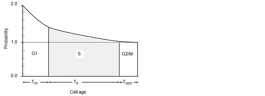
Figure 1. Theoretical age distribution of asynchronous cells throughout the cell cycle.
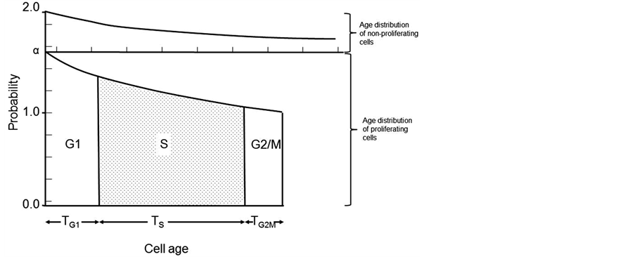
Figure 2. Theoretical age distribution of a cell population containing proliferating and non-proliferating cells.
new non-proliferating cells. This leads to the concept of growth fraction which is used to describe the fraction of cells that are proliferating
 (3)
(3)
 (4)
(4)
The growth fraction can only have a precise meaning when the distinction between proliferating and nonproliferating cells is clearly defined. The calculation of the growth fraction is based upon the relationship
 (5)
(5)
Where LI is the labeling index of the whole population and (LI)p is the labeling index of the proliferating cells.
The age distribution is a crucial link between the time a cell spends in a particular state (or cell cycle phase) and the proportion of cells that will be found in that state. The S-phase area and shape of its upper surface from the DNA histogram will be identical to the upper S-phase boundary of the age distribution diagram (Figure 1) if the rate of DNA synthesis is constant. This explains why rapidly dividing cell lines, such as V79 cells, have a skewed DNA profile as they have more cells in early S than in late S. Thus the shape of the DNA histogram reflects the age distribution and proliferation characteristics of the cell line. Measurements in cell population kinetics fall into two categories 1) measurement of time intervals (intermitotic time, duration of S-phase, potential doubling times etc.) and 2) measurements of numbers of cells (total population size, number in mitosis etc.). The function of the age distribution is to link the two either to calculate one from the other or to test a model population. In populations with growth fractions and when the duration of mitosis Tm is small compared to Tc then:
 (6)
(6)
When α = 2 (exponential growth)
 (7)
(7)
When α = 1 (steady state growth)
 (8)
(8)
In cells containing proliferating and non-proliferating cells it is not usually possible to measure labeling and mitotic indices of cells alone, the measure index usually is a function of the whole population. The link between these indices is the growth fraction
 (9)
(9)
If the duration of S-phase (Ts) and the doubling time of the population (Td) is known, then the LI can be calculated using the following equation
 (10)
(10)
In this equation, λ is a parameter of the age distribution that is a function which varies slowly with population doubling time and with the position of the phase of DNA synthesis within the cell cycle. It’s minimum value is 0.693 and in the unlikely event of the S-phase occurring near the beginning of the cell cycle it could reach a value as high as 1.38 [3] .
Cell loss is a common feature of growing cell populations. Loss can occur in various ways under the broad headings of maturation, death and emigration driven by functions such as differentiation and physiological features such as hypoxia and tumor-associated processes including metastatic spread. If a cell population is not acquiring new cells by immigration then the rate of addition of new cells is equal to the cell birth rate. If cell loss is insignificant in mitosis then
 (11)
(11)
The cell production rate is the rate at which a cell population would be expected to grow if no cell loss occurred. From this an estimate of the time within which the population would be expected to double, or turnover time, can be derived
 (12)
(12)
The turnover time is a quantity that only depends on the cell production rate within a tissue. If non-proliferating cells are not accumulated but are lost at the same rate they are produced, then the population will be held in constant size. The turnover time can be described as the time within which the population would produce a number of cells equal to the number originally present if the absolute cell production rate remained constant. In actual cell systems and particularly tumors, some cells will have shorter intermitotic times than others, and these will be replaced more frequently at the expense of cells that may remain in the population without dividing for many turnover times. In such populations the actual turnover time is the harmonic mean of the intermitotic times of the constituent cells. The alternative to the assumption of constant absolute cell production rate is to assume that the mitotic rate keeps in constant relation to the population size and therefore that growth is exponential. Assuming that the new cells that are produced have the same growth fraction as the population as a whole. In this situation it is possible to calculate a population doubling time that is characteristic of the assumed exponential growth; the potential doubling time (Tpot).
 (13)
(13)
The term potential is used in order to emphasize the assumption of no cell loss. The potential doubling time is always a fraction 0.693 of the turnover time (Figure 3), as a result of the assumption that some of the new cells that are produced will enlarge the proliferating cell population and progressively increase the cell production rate. In any situation where exponential growth is a more reasonable assumption than linear growth the potential doubling time is a better parameter to use. It may be estimated by measurement of the mitotic index and mitotic duration by the stathmokinetic method, or more commonly by the measurement of the thymidine or bromodeoxyuridine LI and the duration of the period of DNA synthesis (Ts) using the relation
 (14)
(14)
If cell loss can be assumed to be random with respect to cell age or proliferative status, then a value for λ can be obtained from the following equation
 (15)
(15)
where
 (16)
(16)
In most situations it is not feasible to accurately measure λ and often a value will be assumed for this parameter based on a priori knowledge of the type of cell population. For research on proliferation in human tumors a value of 0.8 is often assumed [19] . As the growth of a cell population will be governed by the rate of cell production minus the cell loss it can be shown that the cell loss factor (Ø) is
 (17)
(17)
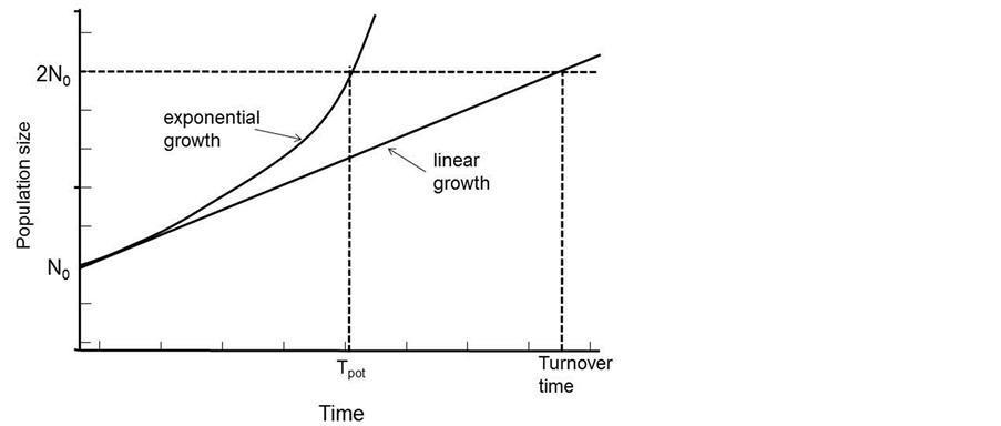
Figure 3. The relationships between the definition of turnover time and potential doubling time.
3. Flow Cytometric Methods to Study Cell Proliferation/Kinetic Parameters
Flow cytometry has the ability to measure several different parameters that relate to the cell cycle and provide different levels of information and sophistication.
3.1. The DNA Profile and S-Phase Fraction
The nuclear DNA content of a cell can be quantitatively measured using fluorescent dyes such as propidium iodide, ethidium bromide or 4’,6-Diamidino-2-Phenylindole, Dilactate (DAPI) that bind stoichiometrically to DNA. Usually the dyes are added to a suspension of permeabilized single cells or nuclei. The principle is that the stained material has incorporated an amount of dye proportional to the amount of DNA. The stained material is then measured in the flow cytometer and the emitted fluorescent signal yields an electronic pulse with a height (amplitude) proportional to the total fluorescence emission from the cell. This staining achieves the fundamental tool of flow cytometric DNA analysis which is the DNA histogram (Figures 4(a)-(c)). The usual flow cytometric procedure involves the exclusion of cell doublets in which two cells with a G1-phase DNA content are recorded by the flow cytometer as one event with a cellular DNA content similar to a G2/M-phase cell. If a sample contains many doublets, this can spuriously increase the relative number of cells in the G2/M-phase of the cell cycle (Figure 4(b)). In order to correct this error, most flow cytometers are equipped with a Doublet Discrimination Module that selects single cells on the basis of pulse processed data. The emitted fluorescent light of the DNA dye (FL2) generates an electronic signal that can be recorded as height (FL2H) for the intensity of the staining as well as measured as pulse-area (FL2A) and pulse-width (FL2W) of the samples. By plotting the FL2W versus FL2A in a dot plot graph a discrimination of a G1 doublet from a G2/M single can be made (Figure 4(a)). The histogram of this gated population (Figure 4(c)) shows the three distinct populations that can be recognized in a proliferating cell population the G0/G1, S, and G2 + M.
The aim of staining protocols is to provide reliable, robust and reproducible methods to produce good quality DNA histograms. A good quality DNA histogram is characterized by a minimal amount of debris and a symmetrical G1 peak with a low coefficient of variation (CV). These attributes facilitate the analysis of the histogram to reliably measure the different components of information present in the profile such as the number of subpopulations with different DNA contents, including their DNA index and their proportion, and the percentages of cells in each phase of the cell cycle (G1, S and G2 + M).
The DNA histogram for cell lines appears as a relatively simple data set which is usually characterized by two peaks separated by a trough. The first peak, which is usually larger, represents cells in G0/G1 and the second, which have twice the fluorescence intensity of the first, corresponds to cells with G2 or M DNA content. The cells between these peaks represent S-phase cells. In an ideal DNA histogram all G0/G1 cells and G2/M cells
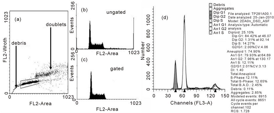
Figure 4. The DNA profile. In a, doublet discrimination using pulse processing is used to clean up the DNA profile. The ungated DNA profile is shown in b whilst the gated profile is shown in c. In d, an example of a human tumor exhibiting aneuploidy is shown with the deconvolution of the profile using ModFit software.
would reside in two single channels as they have the same DNA content. However, in practice the data are distributed due to instrument-related, staining and biological factors, and this dispersion is assumed to be Gaussian.
The shape of the S-phase distribution is an important consideration for the analysis of cell-cycle phase distribution. The dispersion in the DNA histogram requires that statistical models need to be applied to deconvolute the overlap of the S-phase distribution into the G1 and G2 populations. In general Gaussian peaks are fitted to the GI and G2 populations but a variety of models including multiple Gaussians, rectilinear or polynomial have been applied to model different S-phase distributions [20] .
The term ploidy is often used in flow cytometry to describe the quantity of DNA in a sample. However, ploidy is a cytogenetic term referring to the number of chromosomes which are not measured by simple DNA staining and flow cytometric analysis. The term “DNA index” is a more acceptable and realistic description of the information that is obtained from flow cytometric analysis of DNA. The DNA index is the ratio of the G1 peak position of a test population to the G1 peak position of a known diploid standard. The key aspects for rigorous DNA index analysis are the quality of sample preparation, stoichiometry of DNA dye binding and methods of standardization.
There are many different methods for extracting high quality DNA profiles from cells and tissues. The Vindelov technique [21] is widely cited as one of the best techniques to produce DNA profiles with low coefficients of variation on the G1 peak. The production of good quality DNA profiles from cells extracted from solid tumors has always been problematical due to the need to use fresh tissue which is digested by enzymes such as trypsin, collagenase and elastase. A method which we have used extensively with consistent results in terms of yield and DNA staining uses pepsin digestion of 70% ethanol-fixed tumors to produce nuclei [22] . Analysis of the DNA histogram is usually achieved using proprietary software such as ModFit (Figure 4(d)).
Static DNA profiles provide a snapshot of the distribution of cells throughout the cell cycle and large S-phase fractions are indicative of rapidly cycling cell populations whilst small S-phase fractions would be associated with slowly cycling cells. The percent of cells in each cell cycle phase is also indicative of the length of the cell cycle phase relative to the cell cycle time. Experiments involving dynamic changes in DNA profiles following treatment with drugs or other experimental manipulations can reveal information on cell cycle delays. Although more information can be gained using the bromodeoxyuridine method described in the next section.
3.2. The Bromodeoxyuridine Technique
The bromodeoxyuridine (BrdUrd) technique became possible due to the development of monoclonal antibodies that recognise halogenated pyrimidines incorporated into DNA [12] . Dolbeare and colleagues [13] then developed a simultaneous staining method, using FCM, to study the incorporation of BrdUrd relative to DNA content measured by propidium iodide (PI). The general approach to measuring cell kinetics is to identify a “window” in the cell cycle and measure the movement of a cohort of labelled cells through the window. With 3HTdR, the only identifiable window is mitosis; consequently, the percent labelled mitosis (PLM) analysis was developed. However, with the BrdUrd/PI method windows can be set in any phase of the cell cycle (see Figure 5) looking at either the BrdUrd labelled or unlabelled population using appropriate computer-generated regions.
The essence of the procedure is to pulse label with BrdUrd by a short incubation in vitro or by a single injection in vivo, samples are then taken at time intervals thereafter and stained after fixation in ethanol. The cells are stained using a monoclonal antibody against BrdUrd that can either be directly conjugated to a fluorochrome (usually FITC) or alternatively bound to a second antibody conjugated with FITC. The cells are then counterstained with PI to measure DNA content and analysed on the flow cytometer for red (DNA) and green (BrdUrd) fluorescence. The results are displayed as red (x-axis) versus green (y-axis) bivariate distributions.
The incorporation of BrdUrd into cell cultures is usually achieved with 10 - 20 μM BrdUrd for 20 - 30 minutes to achieve a pulse label. The half-life of BrdUrd in rodent and human blood is short, typically 10 to 15 minutes, such that a single intraperitoneal or intravenous injection acts as a pulse-label. In experimental animals the BrdUrd should be made up in 0.9% saline immediately prior to use again taking care to ensure that the drug is in solution. An i.p. injection of 50 - 100 mg/kg is sufficient for pulse labeling; this would normally be made as a 10 mg/ml solution such that 0.05 - 0.1 ml per 10 gm is administered to the animal. In mice, as many as 8 doses of 100 mg/kg have been given over a 24 hour period in continuous labelling studies.
In man, 200 mg in 20 ml of saline as a single intravenous bolus injection over a few minutes has been routinely administered without any adverse toxicity [19] [23] .
Figure 5 shows a series of distributions of DNA (x-axis), and BrdUrd incorporation (y-axis) obtained at hourly
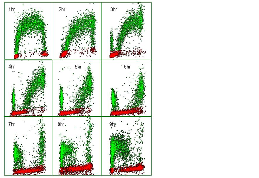
Figure 5. Bivariate distributions of BrdUrd (y-axis) versus DNA content (x-axis) of V79 cells pulse-labeled with 10 μM BrdUrd for 20 minutes and then harvested hourly thereafter.
intervals after pulse labelling V79 Chinese Hamster fibroblasts with 10 µM BrdUrd for 20 minutes in vitro. In the profile recorded after 1 h the BrdUrd labelled S-phase cells are clearly identified by their green fluorescence and lie between the G1 and G2 populations. The latter two populations can also be separately identified by virtue of their lack of BrdUrd uptake and the difference in their DNA content; note that the majority of cells reside in G1. The BrdUrd labelling is classically crescent-shaped with lower levels of uptake in cells that have just entered S-phase from G1 and those found in late S-phase about to enter G2. With time, the profiles show changing patterns. At 2 h, the labelled cohort has become slightly skewed to the right as the cells have made more DNA. One hour later there is the appearance of BrdUrd labelled cells in G1, these represent cells in late S at the time of labelling which have finished S-phase, gone through G2, divided and become two daughter G1 cells. It should also be noted that the original G2 population has also disappeared, as these cells will divide prior to the labelled cells. As time progresses the BrdUrd labelled cohort moves through S-phase and more cells divide. It is also evident that as the original G1 population moves into S-phase; these cells can be identified by virtue of their lack of BrdUrd but they have S-phase DNA. This is another attribute of the technique as each population can be followed as it moves through its cell cycle whether it is BrdUrd labelled or not. Whilst BrdUrd cells reside in G1 they are not making DNA, therefore the number of labelled cells in G1 increases with time until, at 6 h, some of the labelled cells in G1 begin to move into S-phase for the second time as they complete their transit of the G1 phase. This is more evident in the subsequent profiles. Eventually the staining profile will revert to that seen in the 1-hour profile when all cells have completed their cycle; this would probably take 12 h in this particular example.
The basic cell cycle parameters can be calculated by a variety of analyses. The most common method to measure the Tc is to set two narrow windows in mid-S (determined by measuring the mean DNA fluorescence of the G1 and G2 populations). One widow is set in the BrdUrd labelled population only, whilst the other spans both labelled and unlabelled populations (Figure 6(a) and Figure 6(b)). The data is expressed as the ratio of labelled to total cells in mid-S. Initially the ratio should be 1 as all cells should be in the labelled window. This however may not be the case in experimental tumours, as some cells in S-phase do not always incorporate the DNA precursor.
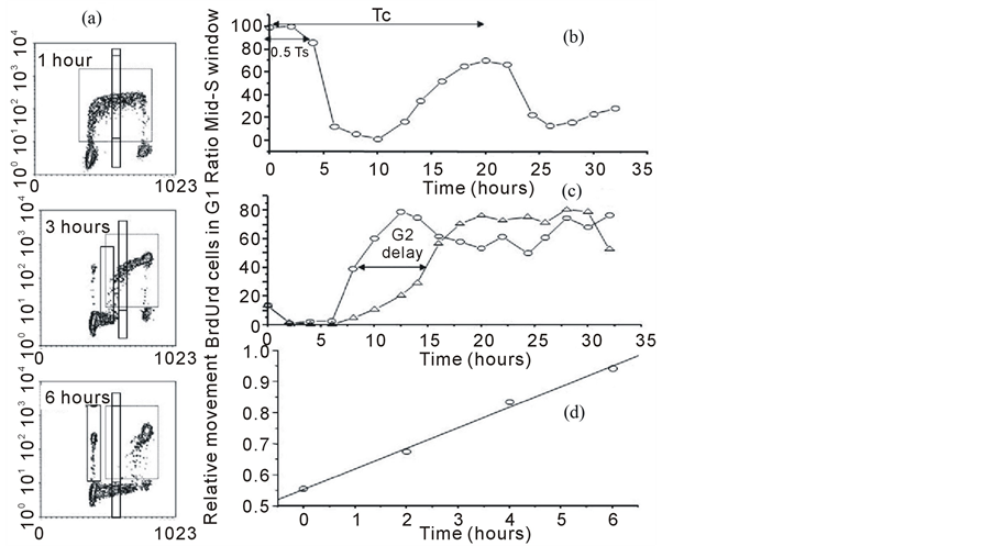
Figure 6. Different methods of analysis to calculate cell kinetic parameters from BrdUrd/DNA profiles. In panel a, a series of profiles are presented at different times after BrdUrd pulse labeling. Different regions of analysis have been superimposed on those profiles. In panel b, the data has been analyzed using two narrow windows in mid-S one of which includes the BrdUrd labeled cells and one which measure unlabeled cells. This creates an analysis similar to pulse-labeled mitosis in which all the basic cell cyle phase transit times can be calculated. In panel c an analysis has been carried out to study G2- phase delays by placing a window in G1 and following the appearance of BrdUrd labeled cells into this region. The BrdUrd labeled cells must transit G2 and mitosis before appearing in this window, so any cell cycle block will delay this appearance. In d, the relative movement analysis is presented which plots the progression of the BrdUrd labeled cells through S-phase (dotted region) relative to the G1 and G2 populations. This analysis can accurately measure Ts and was developed to calculate both Ts and LI from a single delayed time-point after pulse labeling and facilitate the calculation of Tpot in human tumors.
This ratio should remain maximal for a period equal to 0.5 Ts i.e. when the cells in early S-phase at the time of labelling reach the window. The ratio will then fall as the labelled cells clear the region followed by the original (unlabelled) G1 population reaching mid-S. Thus the ratio remains low until the BrdUrd population complete G2, G1 and re-enter S-phase for the second time. At which time the ratio rises and forms a second peak. The mid-point of that second peak is used to determine Tc.
The duration of G2 can be measured from the entry of labelled cells into G1 (Figure 6(a) and Figure 6(c)). This can be achieved by extrapolating a line back to zero which has been fitted to time-points after the first 2 h (because this region may contain cells which are still in early S but are included due to the CV of the G1 population) up until the entry plateaus when all labelled cells are in G1. The data in Figure 6(c) was obtained from primary human fibroblasts cells that were irradiated with 2 Gy of X-rays. At 10 hours after pulse labelling, the BrdUrd labelled cohort, in the control cultures, have either divided and reside in G1 or are in G2 ready to divide. In contrast, the irradiated cells show an almost complete absence of divided BrdUrd labelled cells in G1 because radiation has caused them to accumulate in G2.
The duration of S-phase can be calculated using a technique called “relative movement” (RM) [24] . The procedure is based on a measurement of the mean DNA content of the BrdUrd labelled cells defined by the dotted region in Figure 6(a). Immediately after labelling, the mean of the BrdUrd labelled population is approximately mid-way between G1 and G2, as there is a uniform distribution of cells throughout S-phase. To quantitate the function it is also necessary to measure the mean DNA contents of the G1 and G2 populations (this can be done from the single parameter DNA profile). The RM is calculated by subtracting the mean DNA of the G1 population from that of the labelled cells and dividing it by G1 subtracted from G2. If there is a uniform distribution at time zero, it should give a value of 0.5. With time the mean value of the labelled cohort (which remain undivided) will increase as it progresses through S to G2 (Figure 4(c)). If we make the assumption that the progression through S-phase is linear, a point will be reached when all the labelled cells which remain undivided are in G2; the RM value will equal 1.0 and this time will be equivalent to the Ts as the cells in G2 will have been those in early S at the time of injection. Thus from single or multiple observations, made at a known time greater than G2 but less than Ts + TG2, the Ts can be computed assuming the value is 0.5 at time zero and 1.0 at Ts.
3.3. Cell Proliferation and Cell Cycle-Associated Proteins
Two of the most widely recognized cell proliferation associated proteins are Ki-67 and proliferating cell nuclear antigen (PCNA) [25] . Ki-67 is considered to be a reliable marker distinguishing cycling from noncycling cells and that is often used to measure tumor cells’ growth fraction [26] . PCNA is a multifunctional protein that, among many functions, is a part of the DNA polymerase holoenzyme, interacts with CDKs, cyclins, and CDK inhibitor p21 to form ternary complexes, and participates in nucleotide excision DNA repair. During S phase, PCNA is chromatin-bound, remaining in the nucleus following treatment with detergents.
Figure 7 shows a series of profiles obtained in HT29 human colon carcinoma cells using the described staining protocols. In panel a and b, Ki-67 and total PCNA profiles are shown respectively after methanol fixation of intact cells. In panel a, Ki-67 expression show a gradual increase throughout S phase and is greatest in G2 + M. In G1, there would appear to be a population with slightly higher Ki-67 which may represent recently divided cells, the Ki-67 level then decreases as cells progress through G1 in preparation for S-phase. In this cell line there are no G0 cells; studies using solid tumors and stimulated peripheral blood lymphocytes show a universal lack of Ki-67 in non-cycling cells. In panel B, there is a similar but different expression of total PCNA throughout the cell cycle. There appears to be a much more uniform increase in expression as cells progress from G1 to mitosis without the variation in G1 and G2 + M observed for Ki-67. Although PCNA is synthesized during late G1 and S-phase, it is present throughout the cell cycle due to its long half-life. This characteristic might also result in apparent expression in cells recently leaving the cell cycle and there is also evidence of PCNA expression, in the absence of cell proliferation, in response to growth factors. These properties and the involvement of PCNA in other cellular processes make it a less robust marker of growth fraction than Ki-67. In panel C, the NP40 detergent extraction procedure has been used to demonstrate tightly bound PCNA. The profile resembles that obtained by pulse-labeling with a DNA precursor such as bromodeoxyuridine, in which the S-phase cells have been highlighted by their expression of PCNA at replication sites. This staining technique should provide better functional information concerning the S-phase fraction than single parameter DNA staining. The combi nation of PCNA and Ki-67 staining using a Triton X-100 detergent extraction is shown in panel D. This double staining technique has many advantages, the combination of the two markers allows the investigator to exploit the ability of Ki-67 to discriminate G0 from G1, early G1 from late G1 and G2 and mitosis, whilst PCNA provides the discrimination of S-phase cells. This technique has been used to show that newly recruited cells into the cycle do not express Ki-67 until the end of G1 and is a potentially useful method to study recruitment and repopulation of cells in response to DNA damaging agents.
Immunofluorescent detection of cyclins D, E1, A2, and B1, combined with DNA content measurement, opened a number of new opportunities for probing the cell cycle [27] . It became possible to distinguish G1 cells of higher DNA ploidy from G2 cells of lower DNA ploidy having the same DNA content. It also became possible to discriminate between G2 and M cells, the latter were identified within a well-defined time window between prometaphase and cytokinesis. The lack of cyclin D and cyclin E expression among the cells with G1 content marked the non-cycling G0 cells with hypophosphorylated Rb. Altogether, it become possible to identify cells in six to eight cell cycle compartments differing in their degree of progression through the cycle [27] . Figure 8 shows examples of cyclin A and cyclin E staining versus DNA content (propidium iodide) in unper turbed HT29 colon carcinoma cells. Darzynkiewicz and colleagues have used multiparametric cytometry of cyclins can provide a means to parse cell cycle regulation in fine detail [28] -[33] . Specifically, they have been able to quantify the fraction of cells in G1, S, G2, prophase, prometaphase, metaphase, and late mitosis, and to identify two new cell cycle compartments defined by cytometry. This was accomplished using cyclin markers but also mitotic markers, phospho-histone H3 and MPM-2, which will be described in the next section.
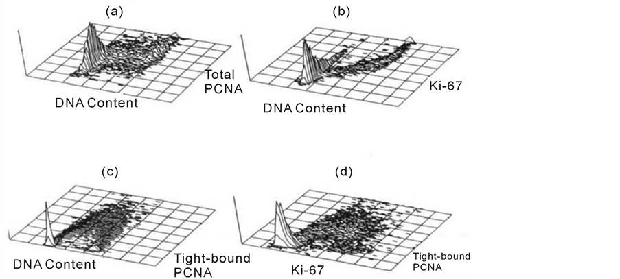
Figure 7. 3-D cytograms the cell proliferation-associated proteins against DNA content (a, b and c) and against each other in d, where the z-axis is cell number.
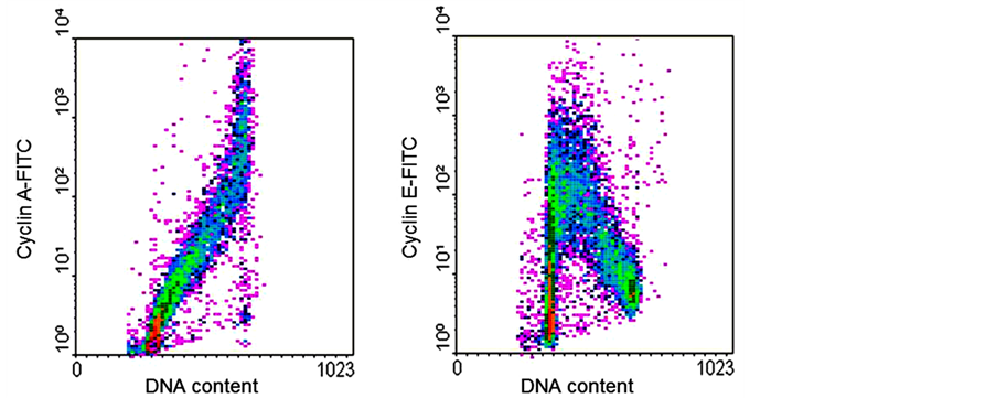
Figure 8. Dot plots of DNA content (x-axis) versuscyclin A or cyclin E (y-axis).
3.4. Mitosis-Associated Proteins
Many epitopes are phosphorylated during mitosis. These epitopes are useful biomarkers for mitotic cells. The most commonly used are MPM-2 and serine 10 of histone H3 (pH3). Histone H3 is phosphorylated at Ser-10 by Aurora B kinase [34] , and appears to be the best marker for mitosis [35] . A typical bivariate dotplot for pH3 versus DNA is presented in Figure 9 where the mitotic population is identified by their increased staining of pH3 within the G2 + M population of the DNA profile. MPM-2 is also a phospho-epitope, which is expressed at a high level on many different proteins in mitosis [36] . Expression of this epitope increases later than phosphorylation of Ser-10 of histone H3 (pH3), and the cytometry of MPM-2 and pH3 as well as an antibody generated against a phospho peptide matching residues 774 - 788 of the human retinoblastoma protein 1 [37] have defined a new cell cycle compartment located past G2 and prior to a cytometrically defined transition state that corresponds to prophase. Prophase cells are characterized by peak or near peak levels of cyclin A and cyclin B1 [38] . The switch from prophase to metaphase is characterized by the activity of a form of the anaphase promoting complex (APC) that degrades cyclin A and, as a result, prometaphase cells can be detected as cells with lower levels of cyclin A, but peak or near peak levels of cyclin B1. The detection of metaphase is defined by undetectable cyclin A but peak levels of cyclin B1. Cyclin B1 accumulates until metaphase and is destroyed by APC at the onset of anaphase [39] . Events after metaphase are not easily resolved using flow cytometry.
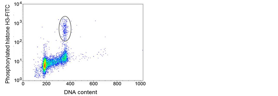
Figure 9. Dot plot of DNA content (x-axis) versusphosphorylated Histone H3 (y-axis).
4. Concluding Statement
Multiparameter flow cytometry offers a unique methodology to investigate a variety of cell kinetic-associated parameters ranging from “snapshots” to true kinetic measurements. With the molecular probes of function/activity of individual cell-cycle-related proteins that are now available, there is a further scope to study the fine detail of molecular events in single cells and flow cytometry will continue to be an essential methodology in cell cycle studies accompanying biochemical and molecular methods.
References
- Howard, A. and Pelc, S.R. (1951) Nuclear Incorporation of 32P as Demonstrated by Autoradiographs. Experimental Cell Research, 2, 178-187. http://dx.doi.org/10.1016/0014-4827(51)90083-3
- Howard, A. and Pelc, S.R. (1953) Synthesis of Deoxyribonucleic Acid in Normal and Irradiated Cells and Its Relation to Chromosome Breakage. Heredity, 6, 261-273.
- Steel, G.G. (1977) Growth Kinetics of Tumours. Clarendon Press, Oxford.
- Kamentsky, L.A., Melamed, M.R. and Derman, H. (1965) Spectrophotometer: New Instrument for Ultrarapid Cell Analysis. Science, 150, 630-631. http://dx.doi.org/10.1126/science.150.3696.630
- Kamentsky, L.A. and Melamed, M.R. (1967) Spectrophotometric Cell Sorter. Science, 156, 1364-1365. http://dx.doi.org/10.1126/science.156.3780.1364
- Fulwyler, M.J. (1965) Electronic Separation of Biological Cells by Volume. Science, 150, 910-911. http://dx.doi.org/10.1126/science.150.3698.910
- Van Dilla, M.A., Trujillo, T.T., Mullaney, P.F. and Coulter, J.R. (1969) Cell Microfluorometry: A Method for Rapid Fluorescence Measurement. Science, 163, 1213-1214. http://dx.doi.org/10.1126/science.163.3872.1213
- Dittrich, W. and Gohde, W. (1969) Impulse Fluorometry of Single Cells in Suspension. Zeitschrift für Naturforschung B, 24, 360-361.
- Crissman, H.A. and Tobey, R.A. (1974) Cell-Cycle Analysis in 20 Minutes. Science, 184, 1297-1298. http://dx.doi.org/10.1126/science.184.4143.1297
- Dean, P.N. and Jett, J.H. (1974) Mathematical Analysis of DNA Distributions Derived from Flow Microfluorometry. The Journal of Cell Biology, 60, 523-527.
- Gray, J.W., Bogart, E., Gavel, D.T., George, Y.S. and Moore 2nd, D.H. (1983) Rapid Cell Cycle Analysis. II. Phase Durations and Dispersions from Computer Analysis of RC Curves. Cell and Tissue Kinetics, 16, 457-471.
- Gratzner, H.G. (1982) Monoclonal Antibody to 5-Bromoand 5-Iododeoxyuridine: A New Reagent for Detection of DNA Replication. Science, 218, 474-475. http://dx.doi.org/10.1126/science.7123245
- Dolbeare, F., Gratzner, H., Pallavicini, M.G. and Gray, J.W. (1983) Flow Cytometric Measurement of Total DNA Content and Incorporated Bromodeoxyuridine. Proceedings of the National Academy of Sciences, 80, 5573-5577. http://dx.doi.org/10.1073/pnas.80.18.5573
- Darzynkiewicz, Z., Crissman, H. and Jacobberger, J.W. (2004) Cytometry of the Cell Cycle: Cycling through History. Cytometry A, 58, 21-32. http://dx.doi.org/10.1002/cyto.a.20003
- Steel, G.G. and Lamerton, L.F. (1969) Cell Population Kinetics and Chemotherapy. I. The Kinetics of Tumor Cell Populations. National Cancer Institute Monograph, 30, 29-42.
- Baserga, R. (1969) Biochemical Events in the Cell Cycle. National Cancer Institute Monograph, 30, 1-14.
- Sherr, C.J. (2000) Cell Cycle Control and Cancer. Harvey Lectures, 96, 73-92.
- Wilson, G.D. (2004) Radiation and the Cell Cycle, Revisited. Cancer Metastasis Reviews, 23, 209-225. http://dx.doi.org/10.1023/B:CANC.0000031762.91306.b4
- Rew, D.A. and Wilson, G.D. (2000) Cell Production Rates in Human Tissues and Tumours and Their Significance. Part 1: An Introduction to the Techniques of Measurement and Their Limitations. European Journal of Surgical Oncology: The Journal of the European Society of Surgical Oncology and the British Association of Surgical Oncology, 26, 227-238.
- Gray, J.W., Dolbeare, F., Pallavicini, M.G., Beisker, W. and Waldman, F. (1986) Cell Cycle Analysis Using Flow Cytometry. International Journal of Radiation Biology. Related Studies in Physics, Chemistry, 49, 237-255. http://dx.doi.org/10.1080/09553008514552531
- Vindelov, L. and Christensen, I.J. (1990) An Integrated Set of Methods for Routine Flow Cytometric DNA Analysis. Methods in Cell Biology, 33, 127-137. http://dx.doi.org/10.1016/S0091-679X(08)60519-1
- Wilson, G.D. (2000) Analysis of DNA-Measurement of Cell Kinetics by the Bromodeoxyuridine/Anti-Bromodeoxyuridine Method. In: Ormerod, M.G., Ed., Flow Cytometry: A Practical Approach, IRL Press, Oxford, 159-177.
- Rew, D.A. and Wilson, G.D. (2000) Cell Production Rates in Human Tissues and Tumours and Their Significance. Part II: Clinical Data. European Journal of Surgical Oncology: The Journal of the European Society of Surgical Oncology and the British Association of Surgical Oncology, 26, 405-417.
- Begg, A.C., McNally, N.J., Shrieve, D.C. and Karcher, H. (1985) A Method to Measure the Duration of DNA Synthesis and the Potential Doubling Time from a Single Sample. Cytometry, 6, 620-626. http://dx.doi.org/10.1002/cyto.990060618
- Wilson, G.D. (1998) Flow Cytometric Detection of Proliferation-Associated Antigens, PCNA and Ki-67. Methods in Molecular Biology, 80, 355-363. http://dx.doi.org/10.1007/978-1-59259-257-9_36
- Gerdes, J., Lemke, H., Baisch, H., Wacker, H.H., Schwab, U. and Stein, H. (1984) Cell Cycle Analysis of a Cell Proliferation-Associated Human Nuclear Antigen Defined by the Monoclonal Antibody Ki-67. Journal of Immunology, 133, 1710-1715.
- Darzynkiewicz, Z., Gong, J., Juan, G., Ardelt, B. and Traganos, F. (1996) Cytometry of Cyclin Proteins. Cytometry, 25, 1-13. http://dx.doi.org/10.1002/(SICI)1097-0320(19960901)25:1<1::AID-CYTO1>3.0.CO;2-N
- Darzynkiewicz, Z., Gong, J. and Traganos, F. (1994) Analysis of DNA Content and Cyclin Protein Expression in Studies of DNA Ploidy, Growth Fraction, Lymphocyte Stimulation, and the Cell Cycle. Methods in Cell Biology, 41, 421-435. http://dx.doi.org/10.1016/S0091-679X(08)61732-X
- Gong, J., Ardelt, B., Traganos, F. and Darzynkiewicz, Z. (1994) Unscheduled Expression of Cyclin B1 and Cyclin E in Several Leukemic and Solid Tumor Cell Lines. Cancer Research, 54, 4285-4288.
- Gong, J., Traganos, F. and Darzynkiewicz, Z. (1993) Simultaneous Analysis of Cell Cycle Kinetics at Two Different DNA Ploidy Levels Based on DNA Content and Cyclin B Measurements. Cancer Research, 53, 5096-5099.
- Gong, J., Traganos, F. and Darzynkiewicz, Z. (1994) Staurosporine Blocks Cell Progression through G1 between the Cyclin D and Cyclin E Restriction Points. Cancer Research, 54, 3136-3139.
- Gong, J., Traganos, F. and Darzynkiewicz, Z. (1995) Threshold Expression of Cyclin E But Not D Type Cyclins Characterizes Normal and Tumour Cells Entering S Phase. Cell Proliferation, 28, 337-346. http://dx.doi.org/10.1111/j.1365-2184.1995.tb00075.x
- Juan, G. and Darzynkiewicz, Z. (2001) Bivariate Analysis of DNA Content and Expression of Cyclin Proteins. Current Protocols in Cytometry, Chapter 7, Unit 7.9.
- Crosio, C., Fimia, G.M., Loury, R., Kimura, M., Okano, Y., Zhou, H., et al. (2002) Mitotic Phosphorylation of Histone H3: Spatio-Temporal Regulation by Mammalian Aurora Kinases. Molecular and Cellular Biology, 22, 874-885. http://dx.doi.org/10.1128/MCB.22.3.874-885.2002
- Juan, G., Traganos, F., James, W.M., Ray, J.M., Roberge, M., Sauve, D.M., et al. (1998) Histone H3 Phosphorylation and Expression of Cyclins A and B1 Measured in Individual Cells during Their Progression through G2 and Mitosis. Cytometry, 32, 71-77. http://dx.doi.org/10.1002/(SICI)1097-0320(19980601)32:2<71::AID-CYTO1>3.0.CO;2-H
- Friedrich, T.D., Okubo, E., Laffin, J. and Lehman, J.M. (1998) Okadaic Acid Induces Appearance of the Mitotic Epitope MPM-2 in SV40-Infected CV-1 Cells with a >G2-Phase DNA Content. Cytometry, 31, 260-264. http://dx.doi.org/10.1002/(SICI)1097-0320(19980401)31:4<260::AID-CYTO5>3.0.CO;2-N
- Jacobberger, J.W., Frisa, P.S., Sramkoski, R.M., Stefan, T., Shults, K.E. and Soni, D.V. (2008) A New Biomarker for Mitotic Cells. Cytometry A, 73, 5-15. http://dx.doi.org/10.1002/cyto.a.20501
- den Elzen, N. and Pines, J. (2001) Cyclin A Is Destroyed in Prometaphase and Can Delay Chromosome Alignment and Anaphase. The Journal of Cell Biology, 153, 121-136. http://dx.doi.org/10.1083/jcb.153.1.121
- Parry, D.H. and O’Farrell, P.H. (2001) The Schedule of Destruction of Three Mitotic Cyclins Can Dictate the Timing of Events during Exit from Mitosis. Current Biology: CB, 11, 671-683. http://dx.doi.org/10.1016/S0960-9822(01)00204-4