Intelligent Information Management
Vol.2 No.3(2010), Article ID:1487,7 pages DOI:10.4236/iim.2012.23026
An Evolutionary Algorithm with Multi-Local Search for the Resource-Constrained Project Scheduling Problem
Department of Industrial Engineering and Management, Yuan Ze University, Jongli City, Taiwan, China
E-mail: s948907@mail.yzu.edu.tw, iehshsu@saturn.yzu.edu.tw
Received November 20, 2009; revised December 25, 2009; accepted January 31, 2010
Keywords: Resource-Constrained Project Scheduling, Evolutionary Algorithms, Local Search, Hybridization
Abstract
This paper introduces a hybrid evolutionary algorithm for the resource-constrained project scheduling problem (RCPSP). Given an RCPSP instance, the algorithm identifies the problem structure and selects a suitable decoding scheme. Then a multi-pass biased sampling method followed up by a multi-local search is used to generate a diverse and good quality initial population. The population then evolves through modified order-based recombination and mutation operators to perform exploration for promising solutions within the entire region. Mutation is performed only if the current population has converged or the produced offspring by recombination operator is too similar to one of his parents. Finally the algorithm performs an intensified local search on the best solution found in the evolutionary stage. Computational experiments using standard instances indicate that the proposed algorithm works well in both computational time and solution quality.
1. Introduction (Heading 1)
The resource-constrained project scheduling problem (RCPSP) has applications in many situations such as plant construction, facility and equipment maintenance, new technology or product development. This problem has drawn many researchers’ interest over years due to its wide applications and academic attractiveness. The resource-constrained project scheduling problem can be stated as follows. A project consists of a set N = {0,1,…, J+1} of activities (nodes), where activities 0 and J+1 are dummy and represent the events of the start time and the completion time of the project, respectively. A set of precedence relationships (arcs) between pairs of activities must be specified in the project. These activities and their associated precedence relationships can be represented by an acyclic directed network G = (N, A), where A is the set of arcs. In an acyclic directed network, there exists a topological ordering on nodes such that no node is numbered smaller than any of its predecessors. An activity list (AL) is a sequence of the activities that follows the precedence constraints; thus, it is a type of topological ordering.
In the study, each activity has to be processed without interruption to complete the project. The processing time (duration) of an activity j is denoted by dj, and its request for resource type k is rjk. For the dummy activities, d0 = dJ+1 = 0, and  =
=  = 0, for any resource type k. The availability of each resource type k in each time period is Rk units, k = 1,…,K. A project schedule S can be represented by the start time of each activity,
  with
with  and
and  = project makespan, or finish time of each activity, (f0, f1,…,fJ+1) with f0 = 0 and fJ + 1 = sJ + 1. Note that
  for all j. A schedule S is feasible if it satisfies both precedence and resource constraints at any execution time period. The objective of the RCPSP is to determine a feasible schedule S with minimum project makespan.
The optimization of this problem is NP-hard in the strong sense [1]. For information about the RCPSP problem classification and algorithm performance, we refer to the surveys provided by [2,3]. In producing feasible schedules, serial schedule generation scheme (SSGS) and parallel schedule generation scheme (P-SGS) are usually used. Kolish [4] showed that S-SGS generates active schedules, whereas P-SGS generates nondelay schedules. The set of non-delay schedules is a subset of active schedules and an optimal schedule is an active schedule. The experimental results also indicate that for small size problems and hard problems (scarce resource and/or large average number of resource types used per activity), P-SGS outperforms S-SGS in solution quality. However, the results are the opposite for large size problems and easy problems.
Roughly speaking, the problem solving approach to RCPSP can be classified into three categories: 1) exact method, 2) X-pass method, and 3) meta-heuristics. Brucker et al. [2] proposed a branch and bound algorithm for solving the RCPSP with branching scheme based on conjunctions (precedence constraints) and disjunctions (induced by the resource constraints). Their computational results using a SUN/Sparc 20/181 workstation within one minute CPU time show that the algorithm solves optimally 425/480 and 326/480 for the 480 PROGEN-instances with J = 30, K = 4 and J = 60, K = 4, respectively. Other exact methods developed by Mingozzi et al. [5] and Donrndorf et al. [6] also reported satisfactory results for the problems with sizes up to 30 activities. For large problem-sized RCPSP instances, the other two approaches seem to be appropriate. These approaches attempt to find an optimal or near-optimal solution within a reasonable time frame.
X-pass method includes single-pass method, biased sampling method, multi-pass method, and adaptive sampling method. While the first two methods obtain their solutions based on one priority rule, multi-pass method chooses the best solution among multiple priority rules, and adaptive sampling method selects a biased sampling method according to problem parameters [7,8]. For detailed discussion on X-pass method, we refer to [3,4]. Klein [9] proposed a variant of X-pass method, which is a priority-rule based bidirectional planning SGS. The experimental results based on the SMFF 360 instances show that this method outperforms forward SGS and backward SGS. In the first step of the bidirectional planning method, two partial schedules are produced by a forward SGS and a backward SGS, respectively. Then the two partial schedules are merged into a single complete schedule as follows: first, sort the activities of the backward partial schedule in decreasing order according to the latest start times; then, based on this sequence, shift these activities to their earliest start time available in the forward partial schedule. The bidirectional planning strategy will obtain active schedules even if P-SGS is applied. Tormos and Lova [10] reported that X-pass method with forward-backward pass local search can produce very promising results.
Recently, most researchers are employing meta-heuristics for solving the RCPSP. Meta-heuristics have been reported to outperform the priority rule-based algorithms in terms of solution quality, but they require more computational effort. This is because meta-heuristics are capable of searching good solutions in a much larger solution space and exploiting further on the neighboring areas of these good solutions. Some notable meta-heuristics for the RCPSP are tabu algorithms [11], genetic algorithms [12, 13], ant colony optimization [14], simulated annealing [15], variable neighborhood search [16], scatter search + path relinking [17], scatter search + electromagnetism [18]. Valls et al. [19] conducted an experiment to show that the forward-backward pass local search is a simple useful technique that can be easily incorporated into diverse algorithms for the RCPSP. For information about the algorithm performance of the RCPSP, we refer to [20].
The remainder of the paper is organized as follows. In Section 2, we present the evolutionary algorithm with multi-local search for solving the RCPSP. Subsequently, we will describe the adaptive decoding schemes, evolutionary operators and several local search used in the algorithm. Section 3 summarizes our numerical results and compares them with the other best known heuristics from the literature. Section 4 concludes the paper with a general discussion of the proposed algorithm as well as a few remarks on future research perspectives.
2. The Algorithm (Heading 1)
The specific parts of the algorithms are representation of the individuals, adaptive decoding schemes, initial populations, genetic operators, and local search. Figure 1 presents the basic scheme of the evolutionary algorithm with multi-local search (EA-MLS).
2.1. Basic Scheme
In the algorithm, activity list is used as the representation for the individuals. This type of representation has been proved to be very effective for solving the RCPSP [12, 13]. Four decoding methods are considered: forward serial list scheduling (F-SLS), backward serial list scheduling
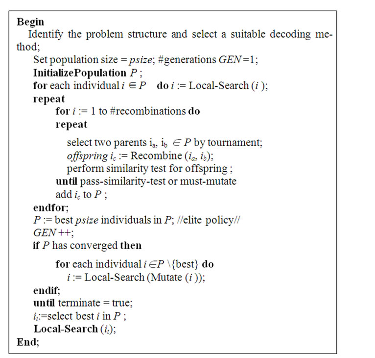
Figure 1. The basic scheme of the EA-MLS algorithm.
(B-SLS), forward parallel list scheduling (F-PLS), and backward parallel list scheduling (B-PLS). In the next section, we will show how to select the suitable decoding method based on an experiment on the PSPLIB j120 instance set.
The initial population is constructed as follows. In order to begin with a diverse population, the individuals are generated by biased sampling methods using four priority rules: latest start time (LST), earliest start time (EST), ACTIM and random. ACTIM determines the longest path from an activity j to the dummy end activity J+1 using activity duration as the distance measure. Each rule contributes to one-fourth of the population size. Once the desired number of feasible solutions is generated, local search procedures are launched to obtain local optima. Each individual is refined by one of the three local searches: individual leftmost move, family leftmost move, and 2-swap.
During the evolutionary phase, modified order-based recombination operator is used to produce offspring. A similarity ratio is applied to test if an offspring is too similar to one of its parents in activity list structure. If the ratio exceeds a preset value, then mutation is performed to produce a significantly different structured activity list. Furthermore, if more than 80% of the individuals in the current population have the same project makespan, then all individuals except the best one are first subject to mutation, and then improved by multi-local search. This adaptive strategy attempts to construct a differently-structured diverse and elite population, and initiates another evolutionary search. Finally, the best solution found in this evolutionary phase will be further refined by an intensified local search.
2.2. Problem Structure
Kolisch and Sprecher [21] identified the structure of RCPSP by three parameters: Network Complexity (NC), Resource Factor (RF) and Resource Strength (RS), where NC is the average number of direct successors per activity, RF is the average number of resource types used by an activity, and RS is a measure of how the resource limits affects the project completion time (makespan). MathematicallyRF = 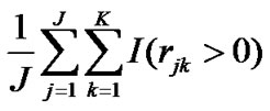 and RS =
 where
where  = 1 if activity j uses resource type k and 0 otherwise,
  represents the maximum usage of resource type k under CPM schedule, and
  is the maximum requirement of resource type k among all activities in the project.
According to these definitions, we can conclude the following:
1) the higher NC value, the more complex the network;
2) the higher RF value, the more types of resource used;
3) the lower RS value, the more scarce the resource. Furthermore, an RCPSP instance with a high RF and low RS is likely to counter resource conflicts, thereby prolonging the project makespan. An RCPSP instance with such structure generally has an optimal project makespan much longer than the same project without the resource constraints. In this paper, we refer to problems with such structure as “hard” and problems with the other structure as “soft”. Kolisch [4] discussed the problems of hard type and suggested that P-SGS be used for such problems.
2.3. Adaptive Decoding Scheme
Four decoding schemes are considered in the EA-MLS: forward SLS, backward SLS, forward PLS, and backward PLS, which are stated as follows, respectively.
Given an activity list (AL) of an RCPSP, AL = , where
  denotes the activity with the jth rank.
1) Forward SLS (F-SLS)
Following the order of activities in AL, the start time of each activity is scheduled as early as possible without violating the precedence and resource constraints. This method generates an alternative for the earliest start and finish times of each activity in the project.
2) Backward SLS (B-SLS)
Reverse the order of the AL and the precedence relationships (directions of arcs in the project network). Apply F-SLS to obtain the makespan T and the earliest start time of each activity si for the reversed project scheduling problem. The latest finish time of activity i for the original project is T – si.
3) Forward PLS (F-PSL)
The method sequentially selects finish times of activities to schedule the start times of next candidate activities. Start with time 0 and find the candidate activities A0. Process the activities in A0 one by one following the order of activities in AL without violating the resource constraints. The next scheduled time is the earliest finish time among activities in A0, and the candidate activities at this time epoch A1 = unprocessed activities in A0 plus the new activities that are qualified to be scheduled (without violating precedence constraints). Continue the same process until all activities in the project are scheduled.
4) Backward PLS (B-PLS)
Apply the same procedure as stated in B-SLS except that SLS is changed to PLS.
F-SLS or B-SLS obtains an active schedule, while F-PLS or B-PLS obtains a non-delay schedule. List scheduling method is different from SGS in when the priority order of activities is determined during the scheduling process. For example, each time an activity is scheduled, S-SGS selects the next activity from the new candidate set according to some rule. On the other hand, SLS first determines an activity list, and then uses the list to schedule the activities. The activity list is a convenient and effective representation for employing meta-heuristics to solve the RCPSP.
Table 1 presents the results of executing EA-MLS with each decoding scheme alone based on 5,000 schedules for each benchmark instance with 120 activities (J120) in PSPLIB (Project Scheduling Problems Library). The performance measure (deviation) and computational time take the average of 10 runs on the test set. We observe that B-SLS and B-PLS outperform the other two decoding schemes in both aspects. Table 2 shows further results that can be used to determine which decoding scheme is suitable for which problem structure. Parameter of RS contains five levels: {0.1, 0.2, …, 0.5} and parameter of RF has four levels: {0.25, 0.50, 0.75, 1}. There is a total of 20 parameter combination levels, with each combination containing 600/20 = 30 instances. Each individual number in Table 2 represents the number of instances in which B-SLS is superior to B-PLS deducting the number of instances in which B-PLS outperforms B-SLS. The comparison for each instance is based on the average of the deviations from the CPM lower bound in the ten runs. The experimental result suggests that B-PLS be the decoding scheme when 0.1 £ RS £ 0.3 and 0.75 £ RF £ 1.0. B-SLS is suggested to be used for the other parameter combination levels. The test environment is described in Section 3.
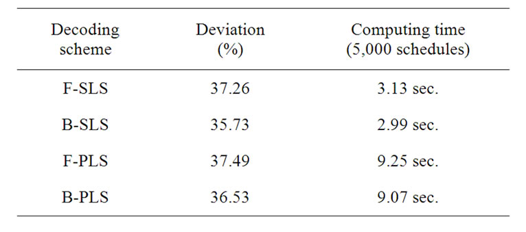
Table 1. Average deviation from CPM lower bound by four decoding methods (J120, PSPLIB).
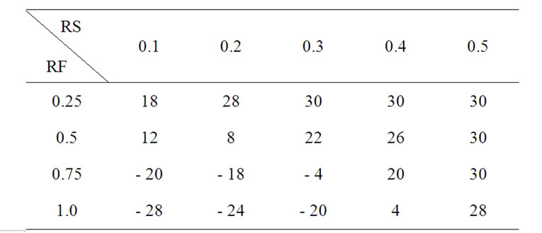
Table 2. Experimental results for performance comparison between B-SLS and B-PLS.
2.4. Genetic Operators
For the recombination operator, two parents ( ,
, ) are selected by tournament method and an offspring is generated. The recombination is performed by a modified order-based procedure in which a number of activities are selected at random from one parent, and then these selected activities are copied into the offspring on the positions where the same activities of the other parent are located. The remaining empty positions of the offspring are sequentially filled with the unselected activities according to the order of the second parent. Next, the precedence feasibility of the offspring is checked. All violated activities are shifted leftward one by one to their first feasible positions. Finally, a similarity ratio test is performed to check if the offspring is acceptable. The similarity ratio is defined as the total number of activities having identical positions over the total number of real activities. The following figures illustrate the recombination process. Figure 2 depicts the precedence relationships of the example project network. Figure 3 presents how an offspring is produced using the order-based genetic operator. Because there is a precedence violation between activities 6 and 1, activity 1 is moved leftward to the first feasible position, which is in front of activity 6. The similarity ratios in this example are 4/6 and 2/6, respectively.
Mutation changes the structure of an activity by performing a large number of 2-swap. In a 2-swap operation, an activity from the activity list is selected at random and the corresponding left shift and right shift limits are computed, and then another activity within the limits is selected at random. If swapping these two activities does not violate the precedence relation, and if the two activities have different start times in the current schedule, then 2-swap is performed; otherwise, another pair of activities is selected.
One situation for performing mutation is when recombination fails to pass the similarity test for a preset number of times, and the last offspring is subject to mutation. Another situation for performing mutation is when the population has converged; here population convergence is defined as a preset percentage of individuals in the population that have the same makespan. Under such a situation, all individuals but the best one will be subject to a preset number of 2-swaps so that the structure of new population is significantly different from that of the original one. The local search scheme used in the initial population is then applied to the individuals of the new population in order to achieve various local optimums located at different regions (diversification and intensification). In other words, the search direction of the algorithm must change if there is little opportunity to improve the quality of the current population.
2.5. Local Search
In the EA-MLS, local search is used in three situations: (1) generating the initial population, (2) new population generated by mutation operator and (3) refining the final best solution. Three types of network-based local search are considered: individual leftmost move, family leftmost move and 2-swap. We will use the project network in Figure 2 as an example to illustrate these local searches in Figure 4. In the individual leftmost move, an activity is chosen at random; if the start time of the selected activity is different from the finish time of all its direct predecessors, the individual leftmost move is performed; otherwise, another activity is chosen at random. The family leftmost move first selects an activity at random and bundles up this activity with all of its direct predecessors; then the bundled activities are moved leftward together to the most front positions of the activity list. The 2-swap local search was described in Subsection 2.4 for the mutation operator.
3. Computational Results
This section presents the experimental results for EA-MLS. The test set comes from J30, J60 and J120 of the PSPLIB. J30 and J60 contain 480 instances, while J120 contains 600 instances. Each instance set has four resource types. The test environment is as follows: CPU: AMD – 2.4G, RAM: 512 DDR 333, HD: 40G 7200 rpm, OS: Win 2K, Language: Visual C#.Net.
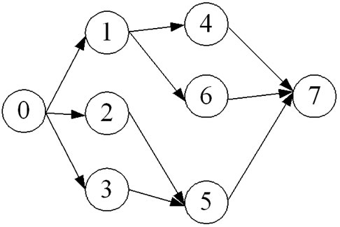
Figure 2. A project network.
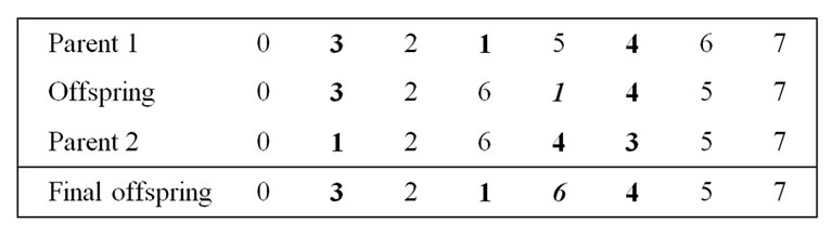
Figure 3. The modified order based recombination operator.
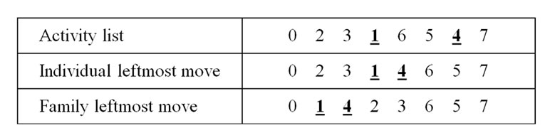
Figure 4. A description of “individual leftmost move” and “family leftmost move”.
Table 3 presents a ten-run performance of EA-MLS on each test set. Table 4 summarizes the experimental results of EA-MLS. We observe that as the problem size grows, the deviation from the optimal value or CPM lower bound increases, and the average number of best solutions obtained decreases. The EA-MLS is a robust algorithm for the RSCPS because the performance of the ten runs deviates very little for each test set. Moreover, the algorithm is capable of getting very good solutions with little computational effort for the problem size within the test set, as is shown by the tables. For the instance set of J30, EA-MLS is superior to the branch and bound algorithm by [2] in terms of finding the total number of optimal solutions and computational efficiency. Tables 5 to 7 compare the performance of the EA-MLS to currently published algorithms using 1,000/ 5,000 schedules as the comparison standard. There are other very good algorithms using different evaluation standards due to their algorithm characteristics. For instance, the VNS by Fleszar and Hindi [16] and the scatter search + path re-linking method by Valls et al. [17]. Tables 5 and 6 show the performance comparison with the EA_MLS and currently published algorithms for the test sets of j30 and j60 based on 1000 schedules and 5000 schedules.
In algorithm EA-MLS, the adaptive decoding scheme is influential in obtaining better quality solutions, as can be observed by Tables 1, 3, and 4. This result is congruent with the performance report of the self-adapting GA proposed by [13], although the adaptive strategies are different. For a given RCPSP instance, the self-adapting GA gradually adjusts the selection of decoding method to the most appropriate one as population evolves. However, our algorithm chooses to determine the decoding method before starting.
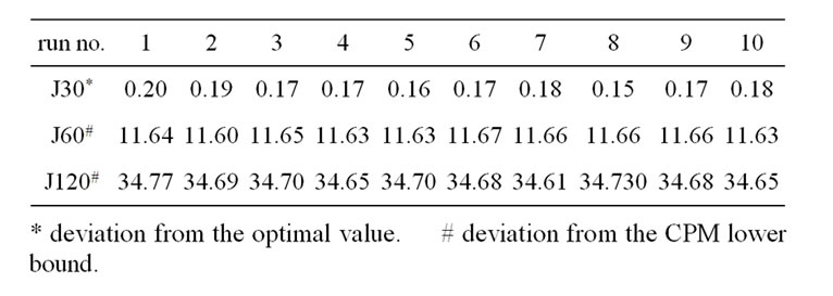
Table 3. Ten run results of EA-MLS on PSPLIB test instance sets (%).
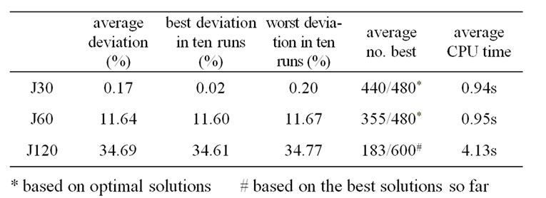
Table 4. Experimental results of EA-MLS on PSPLIB test instance set.
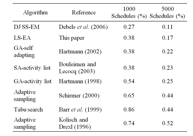
Table 5. Comparison-J30 (480 instances): % above the optimal value.
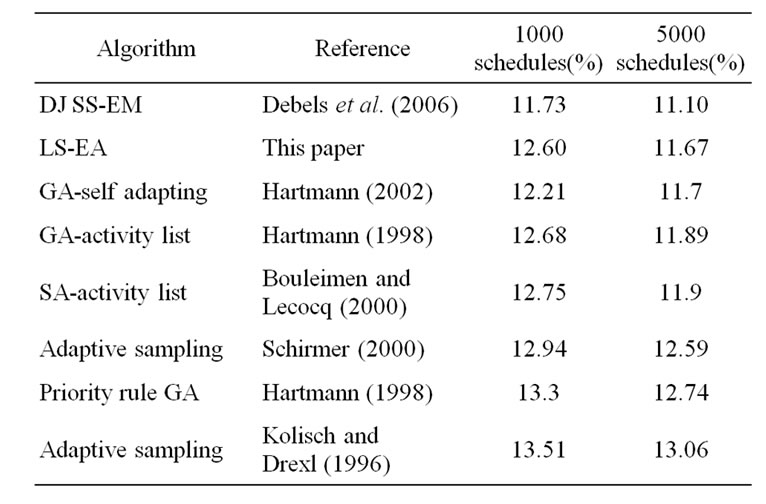
Table 6. Comparison-J60 (480 instances): % above the CPM lower bound.
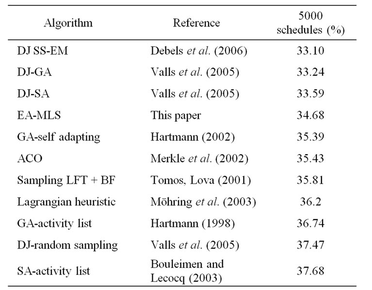
Table 7. Comparison-J120 (600 instances): % above the CPM lower bound.
For the test set of j120, the performance of EA-MLS is inferior to some population based algorithms with the forward-backward double justification (DJ) local search method. In the DJ procedure, the activities of an initial schedule are ranked according to their finish times in decreasing order. Then a new backward schedule is obtained by shifting the activities in the sequence one by one to their latest finish times. In the backward pass, the activities of the new schedule are ranked again according to the latest start time, in increasing order, and then another new schedule is obtained by pushing the activities backward to the earliest start times based on the sequence. The forward-backward pass local search was initiated by [22], and later used by [23] with a different means of implementation. The procedure of Li and Willis is an S-SGS, whereas the procedure of Özdamar and Ulusory is an iterative feature of P-SGS. It is observed that EA-MLS is one of the most competitive algorithms for solving the RCPSP, particularly among algorithms without using the DJ local search. This conclusion is drawn based on the solution quality within 5,000 schedules.
4. Conclusions
This paper proposes a population-based evolutionary algorithm combining the use of a multi-local-search, namely, EA-MLS, for solving the resource-constrained project scheduling problem (RCPSP). The design of the algorithm includes the following characteristics: 1) adaptive decoding scheme, 2) a diverse and elite initial population, 3) a mutation operator for switching the search path to other regions, 4) multi-local search applied at the right timing to obtain various local optima with different local search methods, 5) algorithm parameters and decoding method are set based on experimental analysis. As a result, the EA-MLS is capable of solving the RCPSP efficiently. Although the conclusion is made based on the experiment using PSPLIB J120 instances, we believe that EA-MLS should perform equally well for the other types of RCPSP instances; for example, an RCPSP with various problem sizes and resource types.
We observed by the computational results that the adaptive decoding scheme improves significantly the performance of EA-MLS. Thus, one possibility to promote the performance of EA-MLS is to introduce the bidirectional planning method to the algorithm’s decoding scheme. This bidirectional decoding method possesses the advantage of the forward-backward pass local search and, to the best of our knowledge, has not yet been used in the literature.
In practice, priority rule-based heuristics are in wide and general application because they yield acceptable results with reasonable computational effort. These heuristics are usually contained in commercial software package. However, as computer technology is increasing rapidly nowadays, it is worthwhile to think how to incorporate some high performance meta-heuristics into commercial software, which is capable of solving large and complex project scheduling problems. Many efficient algorithms focus on the objective of minimizing project makespan, regardless of the fact that the schedule generated is a backward one or a forward one. In reality, the project managers are interested in learning the earliest start time (obtained by forward scheduling method), the latest start time (obtained by backward scheduling method), and the slack time of each activity in order to keep good control on project progress. As stated in the previous section, a backward schedule can be transformed with little effort into a forward schedule and may also shorten project makespan.
5. References
[1] J. Blazewicz, J. K. Lenstra, and A. H. G. Rinooy Kan, “Scheduling subject to resource constraints: Classification and complexity,” Discrete Applied Mathematics, Vol. 5, pp. 11–24, 1983.
[2] P. Brucker, A. Drexl, R. Mohring, K. Neumann, and E. Pesch, “Resource-constrained project scheduling: Notation, classification, models, and methods,” European Journal of Operational Research, Vol. 112, pp. 3–41, 1999.
[3] S. Hartmann, and R. Kolisch, “Experimental evaluation of state-of-the-art heuristics for the resource-constrained project scheduling problem,” European Journal of Operational Research, Vol. 127, pp. 394–407, 2000.
[4] R. Kolisch, “Serial and parallel resource-constrained project scheduling problem revisited: Theory and computation,” European Journal of Operational Research, Vol. 90, pp. 320–333, 1996.
[5] A. Minggozzi, V. Maniezzo, S. Ricciardelli, and L. Bianco, “An exact algorithm for project scheduling with resource constraints based on a new mathematical formulation,” Management Science, Vol. 44, pp. 714–729, 1998.
[6] U. Dorndorf, E. Pesch, and T. Phan-Huy, “A branch-andbound algorithm for the resource constrained project scheduling problem,” Mathematical Methods of Operations Research, Vol. 52, pp. 413–439, 2000.
[7]R. Kolisch and A. Drexl, “Adaptive search for solving hard project scheduling problems,” Naval Research Logistics, Vol. 43, pp. 23–40, 1996.
[8] A. Schirmer, “Case-based reasoning and improved adaptive search for project scheduling,” Technical Report 472, Manuskripte aus den Institute fur Betriebswirtschaftslehre der Universität Kiel, 1998.
[9] R. Klein, “Bidirectional planning: Improving priority rule-based heuristics for scheduling resource-constrained projects,” European Journal of Operational Research, Vol. 127, pp. 619–638, 2000.
[10] P. Toromos, and A. Lova, “A competitive heuristic solution technique for resource-constrained project scheduling,” Annals of Operations Research, Vol. 102, pp. 65–81, 2001.
[11] T. Barr, P. Brucker, and S. Knust, “Tabu search algorithms and lower bounds for the resource-constrained project scheduling problem,” in S. Voss, S. Martello, I. Osman, and C. Roucarion (Ed.), Meta-heuristics: Advances and Trends in Local Search Paradigms for Optimization, Norwell, Kluwer, MA, pp. 1–18, 1998.
[12] S. Hartmann, “A competitive genetic algorithm for resource-constrained project scheduling,” Naval Research, Logistics, Vol. 45, pp. 733–750, 1998.
[13; S. Hartmann, “A self-adapting genetic algorithm for project scheduling under resource constraints,” Naval Research Logistics, Vol. 49, pp. 433–448, 2002.
[14] D. Merkle, M. Middendorf, and H. Schmeck, “Ant colony optimization for resource-constrained project scheduling,” IEEE Transactions on Evolutionary Computation, Vol. 6, pp. 333–346, 2002.
[15] K. Bouleimen and H. Lecocq, “A new efficient simulated annealing algorithm for the resource-constrained project scheduling problem and its multiple mode version,” European Journal of Operational Research, Vol. 149, pp. 268–281, 2003.
[16] K. Fleszar and K. Hindi, “Solving the resource-constrained project scheduling problem by a variable neighborhood search,” European Journal of Operational Research, Vol. 155, pp. 402–413, 2004.
[17] V. Valls, F. Ballestin, and S. Quintanilla, “A population-based approach to the resource-constrained project scheduling problem,” Annals of Operations Research, Vol. 131, pp. 305–324, 2004.
[18] D. Debels, B. D. Reyck, R. Leus, and M. Vanhoucke, “A hybrid scatter search/electromagnetism meta-heuristic for project scheduling,” European Journal of Operational Research, Vol. 169, pp. 638–653, 2006.
[19] V. Valls, F. Ballestin, and S. Quintanilla, “Justification and RCPSP: A technique that pays,” European Journal of Operational Research, Vol. 165, pp. 375–386, 2005.
[20] R. Kolisch and S. Hartmann, “Experimental evaluation of state-of-the-art heuristics for the resource-constrained project scheduling: An update,” European Journal of Operational Research, Vol. 174, pp. 23–37, 2006.
[21] R. Kolisch and A. Sprecher, “PSPLIB-A project scheduling problem library,” European Journal of Operational Research, Vol. 96, pp. 205–216. 1996.
[22] K. Y. Li and R. J. Willis, “An iterative scheduling technique for resource constrained project scheduling,” European Journal of Operational Research, Vol. 56, pp. 370–379, 1992.
[23] L. Özdamar and G. Ulusory, “A note on an iterative forward/backward scheduling technique with reference to a procedure by Li and Willis,” European Journal of Operational Research, Vol. 89, pp. 400–407, 1996.