Journal of Geographic Information System
Vol.5 No.4(2013), Article ID:35362,5 pages DOI:10.4236/jgis.2013.54038
Urban Vegetation Mapping from Fused Hyperspectral Image and LiDAR Data with Application to Monitor Urban Tree Heights
Institute of Geography, Department of Earth Science, Graduate School of Science, Tohoku University, Sendai, Japan
Email: fatwa@s.tohoku.ac.jp
Copyright © 2013 Fatwa Ramdani. This is an open access article distributed under the Creative Commons Attribution License, which permits unrestricted use, distribution, and reproduction in any medium, provided the original work is properly cited.
Received May 7, 2013; revised June 7, 2013; accepted July 7, 2013
Keywords: Fusion; LiDAR; Urban Vegetation; Hyperspectral; Mapping
ABSTRACT
Urban vegetations have infinite proven benefits for urban inhabitants including providing shade, improving air quality, and enhancing the look and feel of communities. But creating a complete inventory is a time consuming and resource intensive process. The extraction of urban vegetation is a challenging task, especially to monitor the urban tree heights. In this study we present an efficient extraction method for mapping and monitoring urban tree heights using fused hyperspectral image and LiDAR data. Endmember distribution mapping using the spectral angle mapper technique is employed in this study. High convenience results achieved using fused hyperspectral and LiDAR data from this semiautomatics technique. This method could enable urban community organizations or local governments to mapping and monitoring urban’s tree height and its spatial distribution.
1. Introduction
Remotely-sensed data and imagery provide a comprehensive, scalable means for detecting and quantifying land use land cover (LULC) change, and its use in mapping urban growth, estimating population density, and modelling sustainability and quality of life is becoming increasingly popular as the scale, cost, and spatial-temporal coverage improves [1]. However, the spatial heterogeneity inherent to urban environments represents substantial challenges to discriminating LULC types using remotely sensed data. Spectral mixtures of vegetation and impervious surfaces common in transitory urbanizing landscapes challenge the ability of spectral-based. Standard LULC classification schema for moderate-resolution data at regional and greater scales often lack the specificity (e.g., “mixed” class) and completeness (e.g., “other” class) necessary for accurate representation of complex urbanizing landscapes. Mapping urban vegetation in details is important to understanding the urban green space available for urban inhabitants [2].
The Light Detection and Ranging (LiDAR) and hyperspectral data provide the best opportunity in order to distinguish urban features from urban vegetations (e.g., impervious surface, and vegetated area). LiDAR airborne laser scanner has emerged as an increasingly popular tool for collecting very high-resolution structural data representing the vertical dimension of the Earth’s surface by measuring the travel time of laser pulses between the sensor and earth objects [3].
Reitberg [4] analysed full waveform LiDAR data for tree species classification in the Bavarian Forest National Park in leaf-on and leaf-off conditions for Norway spruces. In urban environments, many researchers have been documenting the advantages of LiDAR and LiDAR-optical fusion data for LULC classification, city 3D modelling, and feature extraction [5-8].
This study examines the advantage of LiDAR and hyperspectral data fusion to improve mapping and monitoring of urban tree heights along different urban features over the University of Houston and the neighbouring urban area, Houston, USA.
2. Data
A hyperspectral image and a LiDAR derived Digital Surface Model (DSM), both at the same spatial resolution (2.5 m). The hyperspectral imagery consists of 144 spectral bands in the 380 nm to 1050 nm region and has been calibrated to at-sensor Spectral Radiance Units (SRU) = µW/(cm2 sr nm). The corresponding co-Registered DSM consists of elevation in meters above sea level (per the Geoid 2012A model). The data were acquired by the NSF-funded Center for Airborne Laser Mapping (NCALM) over the University of Houston campus and the neighbouring urban area (Figure 1) [9].
3. Methodology
Two separate processing steps were considered for the two different data source. 1) For fused data, we firstly fusion LiDAR and hyperspectral data using layer stacking, and employ the following technique:
• Reduce data dimensionality using Minimum Noise Fraction (MNF) transform.
• Select spectral endmember candidates to reduce spatial data dimensionality using Pure Purity Index (PPI).
• Evaluate linearity and select endmembers using n-D visualizer.
• Mapping endmember distribution using Spectral Angel Mapper (SAM) technique.
• Majority/minority analysis.
• Raster-vector conversion.
2) Urban tree heights then extracted from LiDAR data using urban vegetation class vector data as boundary, furthermore only trees with height more than equal to 1 meter and less than 30 meter extracted. We performed heights filtering technique, all return pulses were used, with canopy spacing 1 m, linear interpolation used for this step and finally geo-processing analysis employed to clip only the urban vegetation.
Human involvement appears in order to select the endmembers using a n-D visualizer, therefore this method called semi-automatics technique. Diagram flow of data processing shown in Figure 2.
3.1. Data Fusion
We fused hyperspectral and LiDAR data at single resolutions to assess differences in classification accuracy with only hyperspectral (non-fusion) data. We then subset the three visible bands of hyperspectral-only data (B1, 502.5 nm; B2, 602.6 nm; B3, 697.9 nm) to produce a composite image near-natural color of the study area with an Red-Green-Blue (RGB) combination B1-B2-B3 for visual interpretation using superimposed technique. We subset the study area to only 100 ha enclosed area.
3.2. Calculating Forward MNF Transform
The calculation of the forward MNF transform occurs in two steps. The first step calculates the noise statistics based on a shift difference method. The second step performs the two principal components transformations. The MNF outputs data that has unit variance, isotropic noise
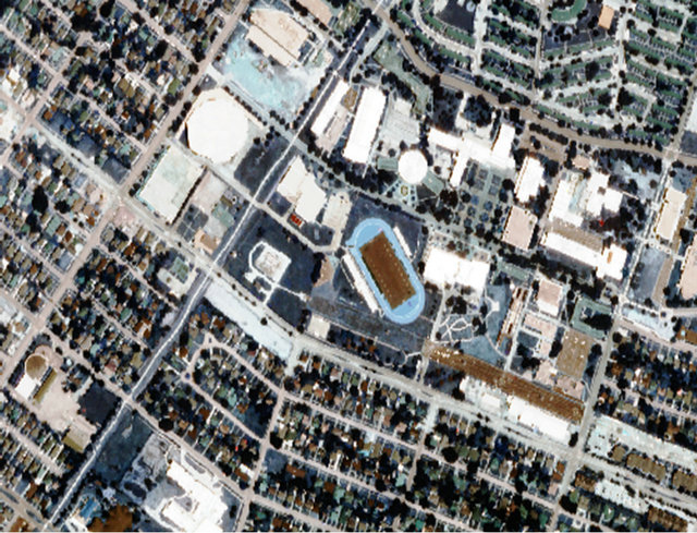
Figure 1. Composite image near-natural color of the study area.
and has decorrelated data sorted by descending variance, the MNF transform will run out of information to process before it runs out of bands, leaving the final MNF output bands as noise-only proof of the hyperspectral nature data [10].
3.3. Pixel Purity Index (PPI)
The Pixel Purity Index (PPI) is used to find the most “spectrally pure” or extreme, pixels in multispectral and hyperspectral data [11]. The most spectrally pure pixels typically correspond to mixing endmembers. The PPI is computed by repeatedly projecting n-dimensional scatter plots onto a random unit vector. The extreme pixels in each projection are recorded and the total number of times each pixel is marked as extreme is noted. The threshold value is used to define how many pixels are marked as extreme at the ends of the projected vector. The threshold value should be approximately 2 - 3 times the noise level in the data (which is 1 when using MNF transformed data). Larger thresholds cause the PPI to find more extreme pixels but they are less likely to be “pure” endmembers [12].
The PPI process exploits convex geometry concepts in the n-dimensional data space of the MNF-processed hyperspectral data. The purest pixels still must be on the extreme corners or edges of the data cloud. While n-dimensional data may be hard to visualize and imagine, the PPI process is relatively insensitive to dimensionality and acts as an n-dimensional “rock tumbler” or “clothes dryer”, tumbling the n-dimensional cloud of data points and counting how many times each pixel is “hit” in this tumbling process. The purer the pixel, the more convex the data cloud is at that location and as a result it will be hit more often and receive a PPI score higher than a lesspure pixel. This convexity concept is based on the assumption of hyperspectral over determinacy [12].
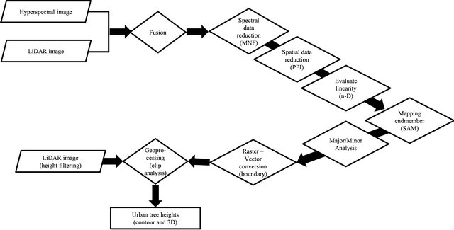
Figure 2. Diagram flow of semi-automatic technique performed in this study.
3.4. n-Dimensional
n-dimensional visualizer provides an interactive tool for finding endmembers by locating and clustering the purest pixels in n-dimensional space. Spectra can be thought of as points in an n-dimensional scatter plot, where “n” is the number of MNF bands or dimensions. The coordinates of each point in n-space consist of “n” values that are simply the spectral radiance or reflectance values in each band for a given pixel [12]. Thus position in the scatterplot conveys the same information as contained in the shape of the spectrum for a single pixel. In n-dimensional scatter plot space, because of the feasibility constraints, the best endmembers occur as vertices, or corners, of an n-Dimensional data cloud or mixing volume. The n-D Visualizer is used to rotate the data cloud, and to locate and highlight the corners of the cloud to find the endmembers [12].
3.5. Spectral Angle Mapper (SAM)
The Spectral Angle Mapper (SAM) matches image spectra to reference spectra in n-dimensions. SAM compares the angle between the endmember spectrum (considered as a n-dimensional vector, where n is the number of bands) and each pixel vector in n-dimensional space. Smaller angles represent closer matches to the reference spectrum. SAM produces a classified image based on the SAM Maximum Angle Threshold. Decreasing this threshold usually results in fewer matching pixels. Increasing this threshold may result in a more spatially coherent image, however, the overall pixel matches will not be as good as for the lower threshold [13].
4. Result and Discussions
It can be seen from n-D visualizer endmember spectra (Figure 3) that wavelength 750 - 800 nm region are sensitive to urban vegetation.
The area of urban vegetation is ~32 ha with height variations ranging from ~12 m to ~30 m. The spatial distribution of higher urban trees is in residential areas, while the lower urban trees spread along the city streets. Figure 4 shows the 3D view of urban tree’s contour extracted from LiDAR data using urban vegetation class vector data as boundary, while Figure 5 shows 3D view of urban tree heights superimposed on near-natural color of the study area.
The small beam may be completely absorbed by the canopy before it reaches the floor and/or may miss the tree tops causing an underestimation of tree height [14].
The basis for LiDAR measurement is that a laser pulse is sent out from the sensor and the leading edge of the returned signal trips a response for a time measurement. The trailing edge of the response is also used to trip a second return time. These are referred to as the “first” and “last” returns. If the first return happens to be associated with a tree canopy top and the last return the underlying ground, then this single signal can be used to provide a measurement of tree height.
Complex backscatter signal (waveform) LiDAR systems typically have a much larger footprint that discrete return systems, being of the order of 10s of metres. This is fundamentally for signal-to-noise reasons: the quantity
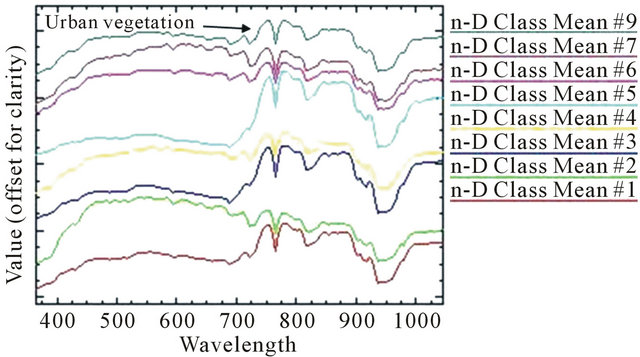
Figure 3. n-D visualizer endmember spectra.
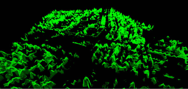
Figure 4. 3D view of urban tree’s contour extracted from LiDAR data using urban vegetation class vector data as boundary.
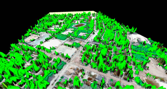
Figure 5. Result, 3D view of urban tree heights superimposed on near-natural color of the study area.
of backscattered energy in a small field of view is low. The energy received per unit time bin is clearly even smaller, so the sensor technologies need to be capable of measuring very low signal levels, very quickly. The LiteMapper-5600 system quotes a waveform sampling interval of 1 ns, giving a multi-target resolution (related to bin size) of better than 0.6 m [15].
This concept can be found in Figure 6, in which we can see that the amplitude of the reflected laser energy shows features that clearly relate in some way to the features of the tree being measured. This study typically observed two main peaks: one associated with the canopy top reflection and one from the ground reflection signal.
The magnitude of the ground reflection signal is gen-
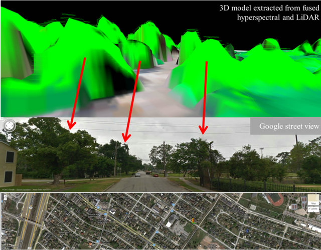
Figure 6. Comparison between 3D model of urban trees extracted from fused hyperspectral and LiDAR data with Google street view. Laser pulses are likely to be reflected by several discrete objects (e.g. leaves, branches, and ground), resulted the urban tree model shows like a cone shape. Location: 29˚43'8.95" North 95˚22'2.12" West.
erally high in urban environment [16], although multiple scattering may increase with the increasing illuminated area, laser pulses are likely to be reflected by several discrete objects (e.g. leaves, branches, and ground), resulted the urban tree model shows like a cone shape. (Figure 6).
This technique allows us to generate the 3D images of the urban vegetation canopy, providing information on tree heights with high accuracy using fused hyperspectral and LiDAR data.
5. Conclusion
We have shown that this study successfully examine the advantage of fused hyperspectral and LiDAR data for mapping and monitoring urban tree heights in convenience yields. This semi-automatics technique gives an efficient framework to be applied for mapping and monitoring urban trees in other cities around the world. However, in this study topography variable is neglected, therefore this method only suitable for the relatively flat urban environment.
6. Acknowledgements
The author would like to thank the Hyperspectral Image Analysis group and the NSF Funded Center for Airborne Laser Mapping (NCALM) at the University of Houston for providing the data sets used in this study, and the IEEE GRSS Data Fusion Technical Committee.
REFERENCES
- J. Rogan and D. M. Chen, “Remote Sensing Technology for Mapping and Monitoring Land-Cover and Land-Use Change,” Progress in Planning, Vol. 61, No. 4, 2004, pp. 301-325. doi:10.1016/S0305-9006(03)00066-7
- F. Ramdani, “Extraction of Urban Vegetation in Highly Dense Urban Environment with Application to Measure Inhabitants’ Satisfaction of Urban Green Space,” Journal of Geographic Information System, Vol. 5, No. 2, 2013, pp. 117-122. doi:10.4236/jgis.2013.52012
- J. R. Jensen, “Remote Sensing of the Environment: An Earth Resource Perspective,” 2nd Edition, Pearson Prentice Hall, Upper Saddle River, 2007.
- J. Reitberg, P. Krzystek and U. Stilla, “Analysis of Full Waveform LIDAR Data for the Classification of Deciduous and Coniferous Trees,” International Journal of Remote Sensing, Vol. 29, No. 5, 2008, pp. 1407-1431. doi:10.1080/01431160701736448
- M. Awrangjeb, M. Ravanbakhsh and C. S. Fraser, “Automatic Detection of Residential Buildings Using LIDAR Data and Multispectral Imagery,” ISPRS Journal of Photogrammetry and Remote Sensing, Vol. 65, No. 5, 2010, pp. 457-467. doi:10.1016/j.isprsjprs.2010.06.001
- Y. H. Chen, W. Su, J. Li and Z. P. Sun, “Hierarchical Object Oriented Classification Using Very High Resolution Imagery and LIDAR Data over Urban Areas,” Advances in Space Research, Vol. 43, No. 7, 2009, pp. 1101-1110. doi:10.1016/j.asr.2008.11.008
- L. Guo, N. Chehata, C. Mallet and S. Boukir, “Relevance of Airborne Lidar and Multispectral Image Data for Urban Scene Classification Using Random Forests,” ISPRS Journal of Photogrammetry and Remote Sensing, Vol. 66, No. 1, 2011, pp. 56-66. doi:10.1016/j.isprsjprs.2010.08.007
- X. L. Meng, L. Wang, J. L. Silvan-Cardenas and N. Currit, “A Multi-Directional Ground Filtering Algorithm for Airborne LIDAR,” ISPRS Journal of Photogrammetry and Remote Sensing, Vol. 64, No. 1, 2009, pp. 117-124. doi:10.1016/j.isprsjprs.2008.09.001
- IEEE GRSS Data Fusion Contest, 2013. http://www.grss-ieee.org/community/technical-committees/data-fusion/
- A. A. Green, M. Berman, P. Switzer and M. D. Craig, “A Transformation for Ordering Multispectral Data in Terms of Image Quality with Implications for Noise Removal,” IEEE Transactions on Geoscience and Remote Sensing, Vol. 26, No. 1, 1988, pp. 65-74. doi:10.1109/36.3001
- J. W. Boardman, F. A. Kruse and R. O. Green, “Mapping Target Signatures via Partial Unmixing of AVIRIS Data: In Summaries,” Fifth JPL Airborne Earth Science Workshop, JPL Publication 95-1, Vol. 1, 1995, pp. 23-26.
- Exelisvis, “ENVI Software Classic Help”.
- F. A. Kruse, A. B. Lefkoff, J. B. Boardman, K. B. Heidebrecht, A. T. Shapiro, P. J. Barloon, and A. F. H. Goetz, “The Spectral Image Processing System (SIPS)—Interactive Visualization and Analysis of Imaging Spectrometer Data,” Remote Sensing of the Environment, Vol. 44, No. 2-3, 1993, pp. 145-163. doi:10.1016/0034-4257(93)90013-N
- D. A. Zimble, D. L. Evans, G. C. Carlson, R. C. Parker, S. C. Grado and P. D. Gerard, “Characterising Vertical Forest Structure Using Small-Footprint Airborne LiDAR,” Remote sensing of Environment, Vol. 87, No. 2-3, 2003, pp. 171-182. doi:10.1016/S0034-4257(03)00139-1
- C. Hug, A. Ullrich and A. Grimm, “LiteMapper-5600—A Waveform-Digitizing LIDAR Terrain and Vegetation Mapping System,” Proceedings of the ISPRS Working Group VIII/2 Laser-Scanners for Forest and Landscape Assessment, Freiburg, International Archives of Photogrammetry, Remote Sensing and Spatial Information Sciences, Vol. 36, 2004.
- C. Mallet, U. Soergel and F. Bretar, “Analysis of FullWaveform LiDAR Data for Classification of Urban Areas,” The International Archives of the Photogrammetry, Remote Sensing and Spatial Information Sciences. Vol. 37, Beijing, 2008. http://www.isprs.org/proceedings/XXXVII/congress/3_pdf/13.pdf
Abbreviations
DSM (Digital Surface Model)
LiDAR (Light Detection and Ranging)
LULC (Land Use Land Cover)
MNF (Minimum Noise Fraction)
NCALM (NSF-Center for Airborne Laser Mapping)
NSF (National Science Foundation)
PPI (Pure Purity Index)
RGB (Red-Green-Blue)
SAM (Spectral Angel Mapper)
SRU (Spectral Radiance Units)