Journal of Geographic Information System
Vol. 4 No. 6 (2012) , Article ID: 26323 , 33 pages DOI:10.4236/jgis.2012.46060
Urban Growth Prediction: A Review of Computational Models and Human Perceptions
State University of New York College of Environmental Science and Forestry, Syracuse, USA
Email: trdimitrios@gmail.com, gmountrakis@esf.edu
Received September 28, 2012; revised October 28, 2012; accepted November 29, 2012
Keywords: Urban Models; Urbanization Prediction; Survey; GIS Modeling; Urban Planning
ABSTRACT
Human population continues to aggregate in urban centers. This inevitably increases the urban footprint with significant consequences for biodiversity, climate, and environmental resources. Urban growth prediction models have been extensively studied with the overarching goal to assist in sustainable management of urban centers. Despite the extensive body of research, these models are not frequently included in the decision making process. This review aims on bringing this gap by analyzing results from a survey investigating developer and user perceptions from the modeling and planning communities, respectively. An overview of existing models, including advantages and limitations, is also provided. A total of 156 manuscripts is identified. Analysis of aggregated statistics indicates that cellular automata are the prevailing modeling technique, present in the majority of published works. There is also a strong preference for local or regional studies, a choice possibly related to data availability. The survey found a strong recognition of the models’ potential in decision making, but also limited agreement that these models actually reach that potential in practice. Collaboration between planning and modeling communities is deemed essential for transitioning models into practice. Data availability is considered a stronger restraining factor by respondents with limited algorithmic experience, which may indicate that model input data are becoming more specialized, thus significantly limiting wide-spread applicability. This review assesses developer and user perceptions and critically discusses existing urban growth prediction models, acting as a reference for future model development. Specific guidelines are provided to facilitate transition of this relatively mature science into decision making activities.
1. Introduction
Urbanization has significantly increased over the last two centuries. In year 1800 only 2% of people lived in cities, while in year 1900 this percent increased to 12%. Recent studies indicate that in year 2008 more than 50% of the world population lived in urban areas, with this percentage expected to reach 75% by year 2030 [1]. It is estimated that global urban land use will increase by at least 430,000 Km2, about the size of Iraq, by 2030 [2]. Urban land cover occupies only 2% or 3% of the earth surface [3], yet it has been recognized that urban growth is associated with many socioeconomic and environmental problems. For example, impervious surfaces that result from urbanization dramatically increase peak discharges associated with storm and snowmelt events, which in turn makes more likely downstream flooding as storm waters exceed stream channel capacities [4]. The alteration of surface materials also changes the amount of solar radiation reflected or absorbed resulting in micro-climate changes through temperature and humidity alterations. These changes contribute to the urban heat island phenomenon, which affects human health and comfort and increases energy demands for cooling [5]. Furthermore, pollutants that are concentrated on urban surfaces degrade the biological, chemical, and physical characteristics of lakes, streams, and estuaries receiving urban runoff leading to aquatic and terrestrial habitat modifications. It is well-documented that indicators related to the biological integrity of streams and riparian habitat are inversely related to the amount of impervious surfaces adjacent to them [6].
Urban modeling studies are currently considered an essential component for numerous complex environmental approaches. For example, urban growth modeling can assist in adaptation and mitigation scenarios with respect to climate change because of the large amounts of air, soil and waste emissions that occur in large cities [7-11]. Furthermore, due to the increasing trend of urbanization along with potential environmental consequences, urban growth modeling appears to have a protagonistic role in urban planning to assist in decisions related to sustainable urban development [12-17].
As a response, the scientific community has developed numerous urban growth prediction models (UGPMs) over the past decades in order to study urban land use dynamics and simulate urban growth. These models, even though they have a common goal, vary widely in underlying methodologies and theoretical assumptions, and spatial/temporal resolutions and extents. Several reviews are available on the subject [18-22]. The motivation behind our work to shine light in a well-known limitation. Currently, a significant gap exists between modeling efforts and their implementations in decision making as urban planners and decision makers have only partially incorporated these research products. To investigate further this issue an online survey was conducted to identify limitations and areas of improvement for future UGPM applicability. Therefore the overarching goal of this paper is not only to provide the necessary framework for future development of accurate UGPMs with the modeling community but also UGPMs that are applicable to urban planning tasks.
In the next section a retrospective summary of existing works is provided acting as a reference for future UGPM development. Additional text in the appendix discusses different data sources for these models (Text S1). The survey is introduced with associated findings followed by an in depth discussion on the current state-of-the-art and potential areas of improvement in all UGPM stages, from data sources, to mathematical modeling choices to modeling characteristics facilitating effortless incorporation to decision making.
2. Urban Growth Prediction Models
Urban Growth Prediction Models (UGPMs) are tasked to capture intrinsic and complex relationships in space and time. The spatial complexity reflects the impact of numerous biophysical and socioeconomic factors and as a result heterogeneous patterns appear across location and scale thus making urban development a dynamic and non-linear process [23]. Temporal complexity presents itself through the prediction difficulty for extended temporal intervals. The urban evolution often implies irreversibility [24,25] therefore, in a changing urban environment, only short term predictions can be securely applied [23].
Furthermore, the dynamic process of urban growth is associated with decision making complexity [12,26,27]. Decisions of urban planners and policy makers are difficult to predict, especially over an extended period of time as they depend on stakeholder needs, economic pressure and relevant legislation.
A plethora of models has been applied to examine urban growth, approaching the problem from diverse views. A wide range of electronic sources was accessed leading to the eventual selection of 156 UGPM manuscripts. For manuscript selection we followed the Quality of Reporting of Systematic reviews and meta-analyses (PRISMA) guidelines [28]. Our analysis collected manuscripts until August 2012. Figure 1 describes the selection process and a detailed PRISMA statement is presented in the Appendix (Table S3). Initially records were identified through electronic searches in relevant databases (e.g. Sciencedirect) and search engines (e.g. Google Scholar). After removing duplicates unrelated records were removed from the list (e.g. records returned from real estate or urban planning manuscripts). At the next screening level manuscripts were excluded falling in three general categories: 1) did not provide a spatially explicit model output (e.g. demographic, population density, econometric modeling manuscripts); 2) did not incorporate an explicit spatially explicit prediction mechanism (e.g. mostly manuscripts detecting urban change using remotely sensed methods); and 3) did not simulate urban change but other land use types (general land use change models without urban change specialization). Manuscripts in the latter case were reviewed in [29]. At the last stage we excluded manuscripts that were deemed relevant but included either only a theoretical component or were a simple application of previously published work.
A summary of the reviewed manuscripts is presented in Figure 2. Several common characteristics are examined. Firstly, in terms of input types there is a prevalence of biophysical or biophysical/socioeconomic inputs (107 manuscripts) followed by land-use inputs. There is also a strong preference to local (64) and regional (67) studies, possibly due to data availability, development and validation costs and funding directions. The spatial resolution, defined as the cell size of model output (not model inputs), showed a preference for moderate values (<100 m). The temporal resolution, defined as the temporal length of model reference data (not to be confused with prediction temporal extent) showed a tendency for relatively short time intervals (85 manuscripts with <20 years), a constraint possibly imposed by data sources. A summary table for each of the 156 reviewed papers is provided in the Appendix (Tables S1 and S2).
From the modeling perspective two particular decisions significantly affect model design and performance. The first one is conceptual and relates to expected spatial behavior and relationships. The second decision is the underlying algorithmic type for the model. These decisions are discussed in the next two sections.
2.1. Spatial Autocorrelation and Heterogeneity
To address some of the underlying complexities, UGPMs have incorporated two major analytical characteristics of spatial analysis: spatial autocorrelation and spatial heterogeneity. Spatial autocorrelation refers to the systematic
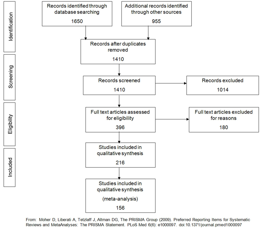
Figure 1. PRISMA 2009 flow diagram regarding the article selection.

Figure 2. Characteristics of reviewed UGPM manuscripts.
variation of a variable, obeying in the first law of Geography [30], in which near things are more related than distant things. According to [31] a spatial or temporal heterogeneous system is characterized by different values in specific locations or time intervals. In an urban environment spatial heterogeneity refers to the different spatial distribution of urbanization along with the underlying driving factors.
Spatial autocorrelation can be described using global and local spatial statistics. In some general spatial statistical studies, global and local spatial statistics have been used, such as: Moran’s I [32-34], Geary C [35-37], G statistic [38,39] and Local Indicators of Spatial Association (LISA) [40,41]. Spatial statistics, such as landscape metrics and texture parameters (e.g. entropy, variance, homogeneity) have been also widely used in urban growth prediction models [42-57].
The estimation of a dependent variable as a function of a matrix of independent variables can be carried out using a) a simple ordinary least-squares (OLS) regression and b) a global spatial regression [58]. The former obeys the Equation (1):
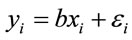 (1)
(1)
where yi is the dependent variable, xi is the matrix of independent variables, b is a vector of coefficient and εi is a vector of random errors. GEOMOD is an example of a land use model which uses multiple regression for determining the weight of each variable in order to specify the location of each changed cell [59]. The global spatial regression is used when there is spatial autocorrelation in the dependent variable and therefore, violation of the OLS regression assumptions is present. Thereupon, a supplementary explanatory variable is added in order to represent the spatial dependency of the dependent variable, as the following Formula (2) illustrates:
 (2)
(2)
where δ is the spatial autoregressive coefficient and wij is the spatial weight of the neighbors i and j [60-63]. Spatial autocorrelation depends on spatial scale [64] and in some cases it is avoided by sampling points at distances greater than the distance where spatial autocorrelation occurs [65]. An alternative solution is autologistic regression that accommodates the autocorrelation effects by using an autocovariate term [66-68]. This additional independent variable captures the spatial variability of the response variable.
Another important characteristic of urban growth is spatial heterogeneity [69]. Different patterns of urban growth may be treated separately using local models instead of a global model into the entire study area [70]. Three modeling techniques may be applied in order to handle spatial heterogeneity: switching regressions, multilevel models and geographically weighted regression [71]. Switching regression model classifies a dataset into a number of mutually exclusive homogenous areas, where a linear regression model is applied in each of them [72,73]. The switching regression model bridges the gap between a local and a global approach in spatial modeling. Multilevel models, also known as hierarchical models, group units of interest (e.g. urban structures) into higher level clusters (e.g. neighborhoods). The motivation of using multilevel models is that they can differentiate heterogeneity between clusters and units nested within clusters [74,75]. Finally, geographically weighted regression is based on assigning weights to all points of dataset according to their distance from a focal point of interest [76].
Despite the fact that these are known issues in UGPMs, from the reviewed manuscripts only six concurrently supported spatial autocorrelation and heterogeneity, and twelve supported either heterogeneity or autocorrelation (Figure 1). The lack of incorporation of these concepts may be attributed to increased mathematical complexity associated with them rather than awareness of their contributions.
2.2. Underlying Modeling Algorithms
As Figure 3 indicates, a wide variety of algorithms has been incorporated in UGPMs with cellular automata tested in the majority of the reviewed manuscripts. In this section we discuss applications, advantages and limitations of currently prevailing and promising methods.
2.2.1 Cellular Automata Modeling
Cellular automata (CA) were introduced by Ulan and Neumann in 1940 and since 1980 numerous models have been developed for simulating urban growth [77]. CA are defined as discrete dynamics systems, represented by a grid of cells, in which local interconnected relationships exhibit global changes [34,78]. Generally, the state of each cell depends on the value of the cell on its previous state as well as the values of its neighbors according to some transition rules. These rules affect the urban growth, indicating environmental and socioeconomic support or limitations.Therefore, the bottom up approach implemented in CA relies on the simulation of local actions that progressively create the global emergent structure [79,80].
CA deals with non-linearity of urban structures and the iterative process leads to produce fractal patterns, which are common characteristics in an urban environment [81].
The applications of CA in urban growth can be classified into: 1) theoretical model developments and 2) applied UGPMs in real data. The first category, which developed in early years of CA, includes theoretical developments
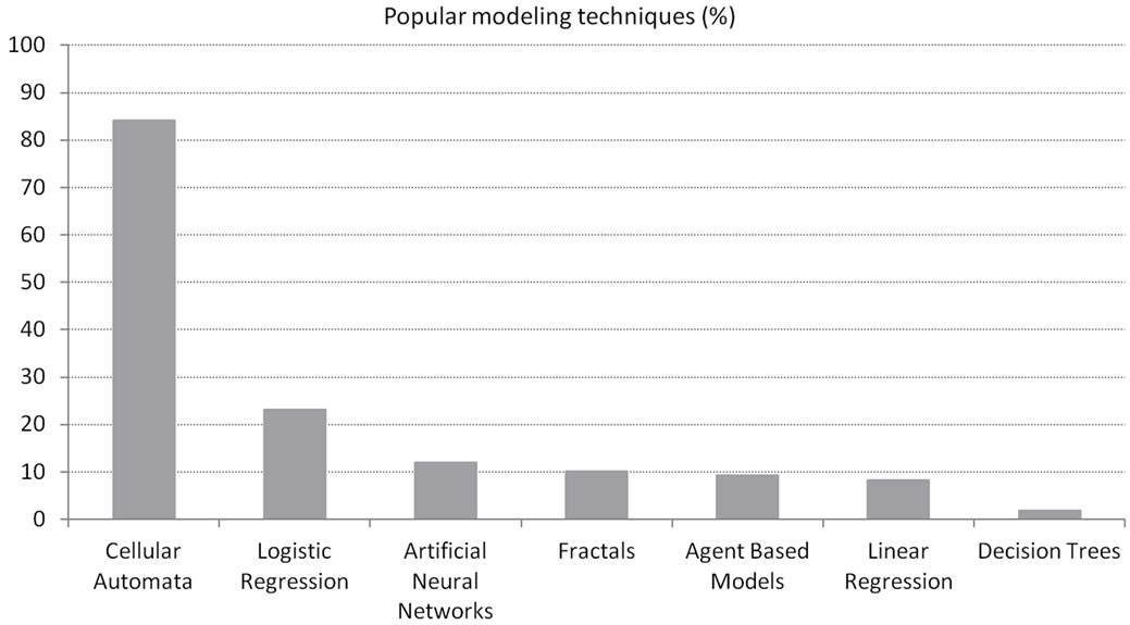
Figure 3. Underlying UGPM algorithms sorted by popularity (percentage of 156 manuscripts, a manuscript may contain multiple algorithms).
of CA models in urban simulation [82-89]. In these studies artificial case exemplars were used to develop theoretical models. The authors also note that urban growth is neither the pure application of The Game of Life nor the pure classical global urban models such as Lowry land use model [34]. Each study area must be examined separately, taking into account the particular conditions which influence urban change. Therefore, a combination of global and local factors must be considered in UGPMs through the appropriate parameterization [84,90,91].
Subsequently, these theoretical approaches found real world implementations. A large number of applications have incorporated CA for UGPM development using real data [91-125]. A combination of CA with Markov models has also appeared in multiple studies [126-130]. A Markov model can not only explain the conversion among land uses, but also calculate the transfer rates among different types. Multi-criteria evaluation techniques [130,131] and weight of evidence [132,133] have been used for estimating the importance of qualitative and quantitative drivers within the CA modelling framework.
An urban growth model, which is widely used by many applications, is the SLEUTH model (slope, landuse, exclusion, urban extent, transportation and hillshade). SLEUTH, introduced in [134], is a CA-based UGPM which uses historical data for calibration of variables, achieving successful implementation in regional scale modeling and ability to deal with protection areas. SLEUTH calibration is a computationally intensive process and therefore requires sufficient computing resources [135]. The SLEUTH model is broadly applied with many study areas found around the globe. Over 100 applications in USA and worldwide were accumulated within ten years [136]. Application examples are available at [137-152]. A new version of the SLEUTH model (SLEUTH-3r) was proposed in [153], increasing the performance and the applicability by introducing new fit statistics, which enhance the calibration process. Metronamica, another CA-based model, was used with SLEUTH in [154]. Metronamica is defined by three components: distance decay functions, integration with GIS and constrained cell transitions by calculating a ranked score for each cell.
Other CA-based urban growth models are iCity and SimLand. iCity (Irregular City), which was developed by [155], is an extension of the traditional form of CA, that includes an irregular lattice [82]. SimLand is a simulation CA model based on multicriteria evaluation methods such as analytical hierarchy process. It was developed by [96] in order to facilitate easier retrieval of spatial data, and to integrate multicriteria evaluation methods and CA with GIS (spatial decision support system), applying a more realistic way in defining transition rules. In addition to the above models, a fuzzy inference guided cellular automata approach has been proposed by [156], where fuzzy theory was applied to provide common semantic and linguistic knowledge to urban growth and simplify transition rules. An optimal combination of transition rules has been investigated using Genetic Algorithms within the calibration process [157,158]. Non-linear transitions rules were also examined using Support Vector Machines [159]. Moreover, Artificial Neural Networks were used to generate conversion probabilities from the initial cell to target land use type. [160] applied a Radial Basis Function Neural Network Model (RBFNN) for this objective. Because Neural Networks cannot explicitly identify the contribution of each variable, less important variables may be included into the model. Due to this limitation, Bayesian Networks were also implemented, where land use drivers have a clear interpretation and the probabilities are easier to understand compared to weights within Neural Networks [161]. The importance of each land use driver (weights) can be also determined using Monte Carlo repetitions [162].
[163] used an Agent Based Model within CA to produce an Entity Based model, in which each household member is considered as a separate entity (agent). The neighborhood infrastructure as well as other neighbor entities contribute to each household behavior. Vector based CA have been also used by [164] to overcome the difficulties with sensitivity to cell size and neighbourhood configuration. They allow the presentation of space by applying vector shapes (polygons), while the neighbourhood is semantically described. More specifically, the neighbourhood changes through time without having a fixed distance delineating it. Finally, in a logistic CA model, proposed by [165,166], the urban growth can be described by a continuous spatial diffusion process where the dependent variable is continuous ranging from 0 to 1.
CA methods also face challenges in urban simulations. Due to spatial heterogeneity, different parts of cities should be addressed by different transition rules. Therefore, global transition rules applied by CA may be inappropriate for modeling cellular space. Furthermore, spatial heterogeneity dictates that neighbourhoods should be described by different shapes and sizes in order to capture better spatial interactions of urban structures. CA methods typically implement regularity in neighbourhoods, limiting modeling capabilities. Finally, disadvantages of CA include the assumption of spatial and temporal invariance for transition rules and the inability of CA to deal with stochastic behaviour [82]. CA examines the synchronous dynamics of urban environment, in essence all cells update simultaneously at each iterative step. Real cities violate this condition because of their chaotic behaviour and therefore, further research in stochastic CA is still needed.
2.2.2 Artificial Neural Networks Modeling
Artificial Neural Networks (ANNs) are incorporated in UGPMs due to their increased modeling capabilities. Unlike most multi-variate modeling techniques, ANNs are not significantly affected by input data relationships, therefore no assumptions about spatial autocorrelation and multi-collinearity must be made. The multi-layerperceptron (MLP) neural network, produced by [167] has gained large applicability. MLP is a system composed by a number of single processing elements, called neurons. The network output is computed using an internal transfer function depends on the input neurons which are connected together with weighted relationships. The ANN learns by the existed input and output data through an iterative way of learning (e.g. back-propagation algorithm). ANNs popularity has substantially increased in recent years due to improved computing power capabilities with applications in many scientific fields [168-170]. Because cities grow in a comprehensive way, the ANNs learning process can produce tools capable to model urban structure complexity [171].
UGPMs often incorporate environmental and socioeconomic variables to simulate the change that has occurred. [172,173] produced the Land Transformation Model (LTM), where GIS and ANNs are combined in order to forecast land use changes, taking into account a variety of social, political and environmental factors. Another approach in urban growth prediction is the ART-MMAP [174], which produces a prediction map under different scenarios, using past information of land use driving forces and socioeconomic data. [175] produced an ANN-based urban growth model in order to estimate future urban growth boundaries and complex geometry of cities, based on factors of urban sprawl such as distances from roads, green spaces, service stations and built areas, elevation, slope and aspect. Another ANN-based urban growth model is proposed by [176] in order to reveal how future urban shape or growth patterns relate to site attributes and reduce the subjectivity in urban growth modeling.
ANNs as a non-parametric technique can successfully capture the spatial heterogeneity [177]. [178] designed a multiple neural network, which allows input data to be automatically reallocated into appropriate neural networks, in order to handle spatial heterogeneity. Furthermore, several neural network algorithms have used fuzzy logic [179,180], multivariate analysis [181] and selforganizing maps [182].
ANNs have been also used for calibration and simulation of CA models in urban studies [183,184]. [183] developed an integration of CA and ANNs in order to simulate land use dynamics, using multiple output neurons. Moreover, [98] introduced a land use simulation model which uses a supervised back-propagation ANN and the generated probabilities were input to a CA model. ANN-based cellular automata models were also applied for urban/non urban cell transitions [184,185].
ANNs have the tendency to overfit data; therefore, the training dataset size should be selected carefully with respect to the number of hidden neurons [186]. A usage of at least 5 to 10 times the training size as are the existed weights is generally accepted [187,188]. The demand of a large training size needed to take advantage of ANNs modeling capabilities often limits UGPM incorporation as training data may not be as widely available. Other typical issues associated with ANNs are the “black-box” behavior which limits understanding of urban evolution, and noise tolerance, especially for small sample sizes.
2.2.3. Fractal Modeling
Fractal geometry has also been used in urban growth simulation. Classical Euclidean geometry is recognized as inadequate to describe the spatiotemporal patterns in nature. [189] introduced fractal geometry and since then a rapid expansion of fractals in many scientific fields has been observed [190]. Cities can be considered as fractal objects, where the interaction of different spatial components can be described by non-linear relationships [81]. Fractal theory deals with the non-linearity of spatial structural complexity, indicating that urban growth conforms to a multiscale spatial self-organization [191-196]. Self-organization is an important process in environmental phenomena. It is based on the ability of the system to organize its components with an internal power support. In self-organized systems, the organization spontaneously increases without being controlled by external force, but it is triggered by internal variation process, which could be fluctuations or noise. The urban environment has unexpected behavior, when some regions are isolated and examined separately. Because any region is a component of the urban self-organized system, it must be treated globally rather than as independent part [3,23,171].
A diffusion-limited aggregation (DLA) method was proposed by [197], where the urban structures were generated in a tree-like form, producing spatial self-similarity in different scales. [81] employed fractal methods to measure the irregularity of urban land parcels, examining the similarity of fractal dimension. [198] applied selfaffine fractal structure in order to explain the complex pattern of urban spatiotemporal evolution, followed by an optimization of urban form using fractal dimension. [195] used a Minkowski dilation in order to detect spatial discontinuity or urban agglomeration and applied a threshold which defines the limit of self similarity of the urban system and stops the dilation process.
Although there has been a tendency to see “fractals everywhere”, many objects cannot be considered true fractals. Natural objects and phenomena are not necessarily described by self-similarity [199]. Numerous algorithms have been programmed in order to calculate the fractal dimension. Fractal dimension measurements have limitations such as: a) different techniques of fractal dimension measurement of the same object may yield to different results, b) objects with different morphological characteristics may share the same fractal dimension and c) objects from the same fractal class may have significantly different fractal dimensions [200]. Therefore, different fractal dimensions may be assigned into an urban structure using various software packages. Moreover, urban structures with different texture may produce similar fractal dimension or urban structures with similar texture may have significantly different fractal dimensions. Finally, accurate fractal modeling is highly dependent on the satisfactory assessment of urban complexity.
2.2.4. Linear/Logistic Regression
Linear regression analysis examines the relationships between urban land uses and independent variables. When the dependent variable is dichotomous, logistic regression can be applied to predict the presence or absence of a characteristic based on a matrix of independent variables. For example, a dichotomous dependent variable can be urban change, where a value of 1 indicates change from non urban to urban and 0 indicates no change. The independent variables can be continuous, categorical, or both. Linear and logistic regression models have been widely used in urban growth modeling, accommodating socio-economic and environmental independent variables [3,44,59,66,72,73,76,177,178,181, 201-217]. CLUE (Conversion of Land Use and its Effects) is a model, which simulates land use changes through a non-spatial demand module and a spatially explicit allocation module [206,218]. For the land use demand model, different modeling approaches can be implemented, ranging from trend extrapolations to more complex economic modeling techniques. In the spatial allocation model, the relationships between land use and independent variables are evaluated using logistic regression. A spatially explicit procedure is used to create the Land Use Scanner model, in which the residential land use demand on spatial units is allocated [219,220]. In the Land Use Scanner model, a logistic regression is applied to empirically specify weights for the preparation of suitability maps.
Land Suitability Index maps were created by [221] using frequency ratio, analytical hierarchy process, logistic regression and ANNs in order to evaluate the performance of each method. The accuracy results did not reveal any important differences among these methods. Regression analysis combined with Markov chains appeared in [222] to study how urban growth relates to landscape change as well as to population growth. Moreover, an enhanced approach in spatial modelling, Geographically Weighted Regression, tackles spatial non-stationarity in regression analysis and the regression coefficients are calculated by spatially dependent weights within a neighbourhood [223-225].
Unfortunately, linear and logistic regressions do not offer high modeling capabilities and they fail to capture non-linearity in the relationships between the dependent and independent variables or to address correlations between independent variables.
2.2.5. Agent-Based Modeling
Agent-based models apply a bottom-up approach to yield better understanding of urban systems by allowing the simulation of individual actions of agents and measurement of the resulting system behaviour [226-229]. Agents are autonomous units, which exchange information with other agents under an interactive communication. The individual behavior of the agents allows the influence of human decision making to be incorporated into the model.
A framework which allows describing urban dynamics as a function of interaction between mobile “agents” and static CA is very important in simulating urban sprawl [230]. [231] developed a national scale simulation agentbased model that was based on applying the concept of the “agent” as the decision maker, taking into account the available biophysical and human factors. A multi-agent model for the study of urbanism is presented by [232], in which different rules and parameters can change the spatial structure of the urban system. Moreover, another multi-agent model is applied by [233] where the interactions of different agents, such as residents, peasants and governments are simulated. A statistical approach in validating spatial patterns in agent-based models is presented by [234]. [235] examined the spread of urban development, evaluating the effectiveness of greenbelts located beside a developed area. [236] developed a model which simulates the polycentric development of urban systems using household agents who choose the location of their houses according to several properties such as land prices, traffic problem, and landscape attractiveness. Despite the satisfactory applicability of agent-based models in urban growth simulation, there are limitations mostly resulting from the arbitrary definitions of initial conditions and interaction rules of agents, which could lead to highly variable results [237].
2.2.6. Decision Trees Modeling
Decision trees is a top-down classification algorithm, which has been used in land use change modeling [44,238,239] and land use classification from remotely sensed imagery [240,241]. Despite their limited use in urban growth modeling, decision trees are of particular interest due to their ability to generate rules and the easiness to understand the model structure. Decision trees automatically derive a hierarchy of partition rules that are used to split data into sequential segments. The construction of a decision tree involves three basic steps. The first step is related with tree building using recursive splitting of nodes. In the second step a pruning process is applied, where smaller trees are produced with lower complexity [242-244]. The reduction of overfitting by removal the noisy and erroneous data is also achieved through a pruning process [245]. Finally, the optimal tree which yields the lower testing error is selected. There are two different types of decision trees according to the learning algorithm: a) classification trees and b) regression trees. In the former, the results of the predicted variable take only two values, usually 0 and 1, while in the latter the predicted output varies between the values of the dependent variable [243]. Decision trees have been widely used in urban land use image-based classification to map urban structures and urban vegetation cover, which are important components in urban modeling and planning [246-249].
Spatial heterogeneity is an important attribute of urban development [69]. An important limitation of decision trees is the simple-algorithm structure, where the entire area is indiscriminately targeted into a global rule. As a result, a low degree of spatial heterogeneity can be incorporated into the model [250]. [70] investigated an expert-based selection of models applied in different regions and the results showed that this approach performs better than using a global model.
Many environmental variables exhibit spatial autocorrelation causing spatial clustering. The spatially dependent data produce less information, making the degrees of freedom of the sample exaggerated [251]. Therefore, spatial autocorrelation causes underperformance of the decision tree modeling [252-254]. However, this limitation could be overcome using a proper sampling design, where the distance between sampling points is greater than the distance at which spatial autocorrelation occurs [255-257]. [258] introduced a novel method in order to handle spatial autocorrelation. According to this method, the conventional entropy of the decision tree was replaced by spatial entropy, which takes into account the spatial autocorrelation.
Unfortunately, decision trees can create over-complex structures that restrict generalization abilities. This issue, known as overfitting, can be rectified to a certain extent using a pruning process. Moreover, decision trees are unstable algorithms as they can produce dramatically different classifiers by using only slightly different training samples [259]. This instability could be reduced by applying a number of decision trees into the training sample each time the training sample changes. Finally, when data includes categorical variables, information achieved from decision trees is biased in favor of the variables with more categories. [260] presents a bias correction to reduce the difference between numerical and categorical variables using a univariate split method based on several aspects of the data such as sample size, number of variables, and missing values.
3. A Survey on Model Integration to Decision Making
The application of urban planning to address issues related to sustainable development represents a balancing act between environmental resources and economic demands. The World Planners Congress in Vancouver in 2006 suggested that urban planners should address urban sustainability in developing and poor countries, putting human livelihoods in the core of urban planning [261]. Because of the increasing trend of urbanization along with potential environmental consequences, urban growth modeling should have a protagonistic role in urban planning to provide appropriate decisions for sustainable urban development [12,13,15,16,262].
However, despite significant efforts in developing UGPMs their usage is limited in the planning community. To investigate further potential reasons that restrict this transition from development to practice a survey was conducted. We are further motivated to use the survey results as a guide for future improvements.
3.1. Questionnaire Content
An online questionnaire was constructed and requested information on the respondent’s background and UGPM development and practise. Table 1 summarizes the questions related to the respondent’s background, such as education (highest degree), employment type and GIS/ professional/policy experience.
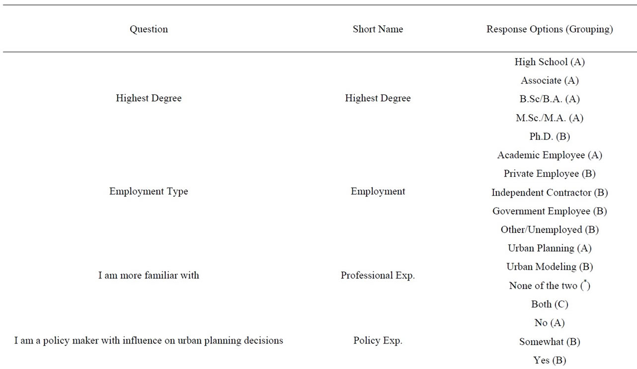
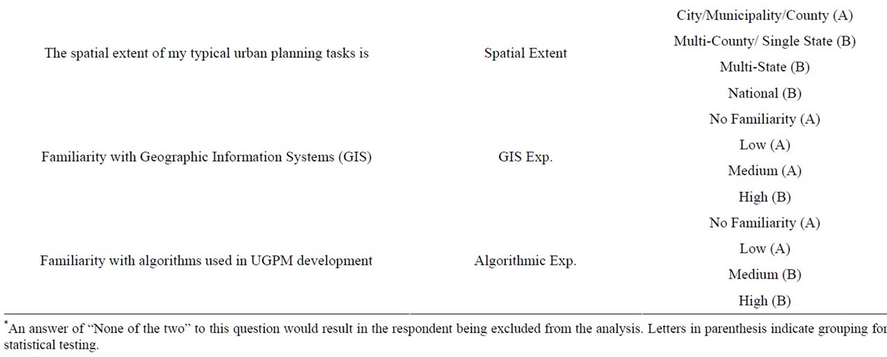
Table 1. Professional background of respondent and corresponding statistical groupings.
Answers to these questions were used initially to screen participants (e.g. those with no relevant experience) and later to identify patterns in subgroup responses (e.g. whether data limitations were more pronounced depending on respondent’s GIS experience).
The second part of the survey requested the respondent’s opinion on UGPM related questions. The question text and answer type along with their short name used in follow up analysis are listed in Table 2.
3.2. Questionnaire Dissemination and Response Rates
The target audience included respondents from both the modeling and planning communities. Modellers were identified through relevant literature manuscripts. Approximately 1000 email addresses were collected. An email was sent out explaining the survey along with a direct link for participation. Responses to the direct link were not tracked as our IRB protocol required complete anonymity but from analyzing the participants’ background the estimated response rate was 14% (app. 140 responses). The access the planning community we solicited help from the American Planning Association. After satisfying their internal review process a direct link of the survey along with a short explanation was included in APA’s electronic newsletter titled APA Interact. The approximate dissemination base was 10,000 members and we estimate 100 responses were obtained leading to a 1% response rate. Considering practical limitations, especially related to privacy, the respondents were deemed a representative sample without a known bias.
In total 242 questionnaires were submitted. After filtering for non-relevant background and those answers belonging to the “Neutral” category the range of usable responses ranged from 84 to 166. Table 3 provides a detailed participation count for each question, also taking account groups outlined in Table 1 as A, B or C.
3.3. Questionnaire Findings
Results are aggregated in Figure 4. There is an overwhelming response in the potential of UGPMs (98% positive), however respondents are split on whether UGPMs currently reach that potential in practice (43% positive). The lack of current widespread implementation does not seem explicitly related to UGPMs prediction quality (67% positive). Rather it is constrained by lack of awareness outside the modeling community (92% negative), which is further supported by lack of communication between modeling and planning communities (94% negative). Modelers are found to create models that are not easy to understand (72% negative, with almost identical responses from the planners (74%) and surprisingly the modelers community (71%)), while planners do not identify clear expectations (81% negative with the mod elers being slightly more negative (87%) than the planners (79%)).
Further analysis was undertaken to reveal patterns associated with the respondent’s background. Table 4 lists the Pearson chi-square tests that were conducted to assess if an association existed between the respondents’

Table 2. Survey questions related to UGPMs development and implementation.

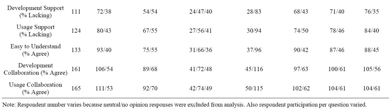
Table 3. Number of respondents per group.
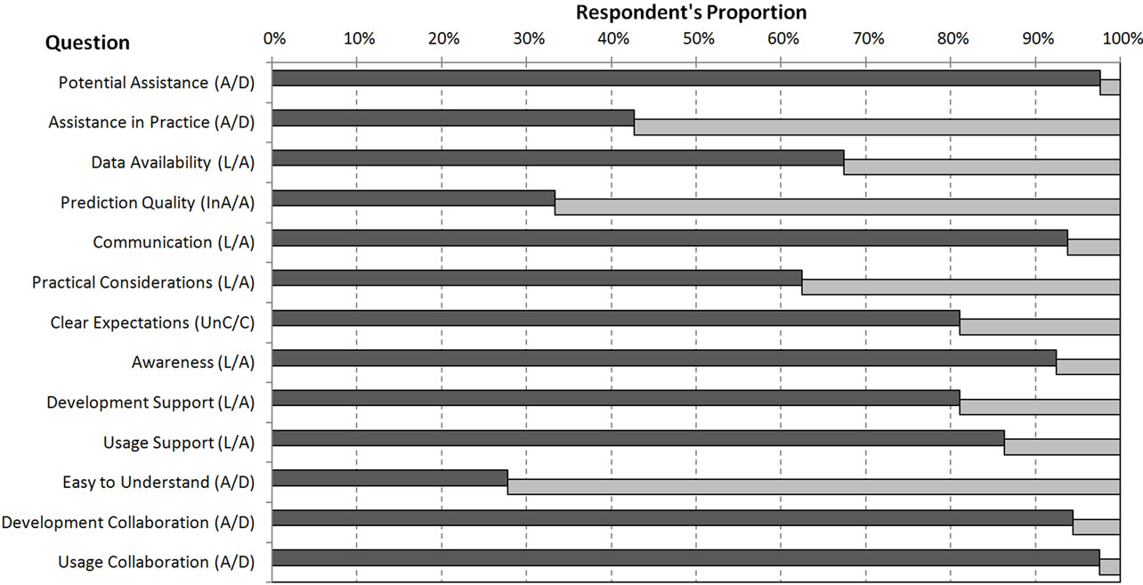
Figure 4. Summary results for survey.

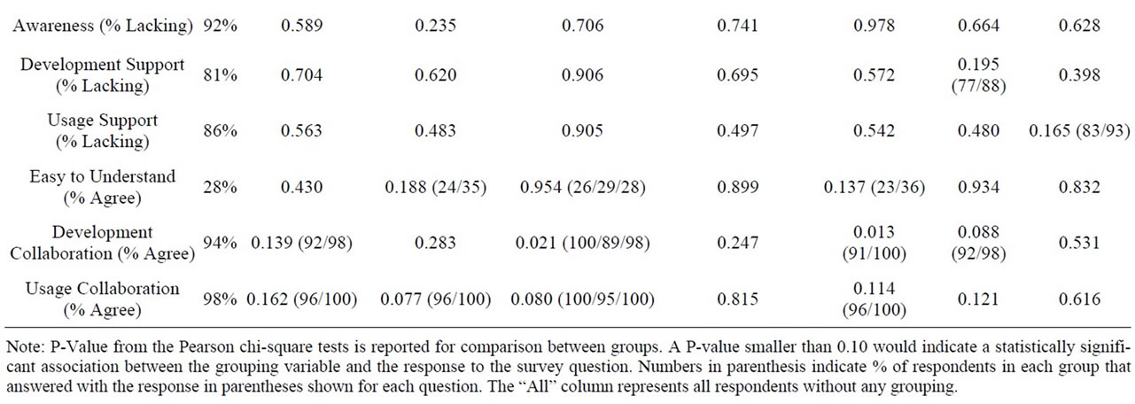
Table 4. Individual question responses for different respondent background groups.
background grouping (A, B or C groups in Table 1) and the response to a survey question (e.g. % Agree or Strongly Agree). For example, if the background group was Highest Degree and the survey question had response options of “agree” and “disagree”, the Pearson test evaluates whether the percent responding “agree” is the same for each of the two Highest Degree groups (PhD/Other). The Pearson tests were conducted using a Type I error rate of 0.10. The highlighted cells in Table 4 correspond to statistically significant differences.
Analysis of the results identified the following interesting findings:
• A surprising result was that respondents with higher involvement in urban growth model development are more satisfied with data availability than others. Respondents with high GIS experience (58%), PhD degrees (63%), academic employment (63%) and large scale studies (59%) identified data availability as lacking or significantly lacking. That percentage was higher for medium or lower GIS experience (87%), non-PhDs (75%), non-academics (74%) and respondents with no or low algorithmic experience (80%). Policy experience did not seem to matter (67% for both respondent groups, namely with or without relevant experience).
• On the question regarding whether UGPMs reach their potential in practice, respondents with no policy experience agreed or strongly agreed at a lower percentage than respondents with policy experience (37% vs. 53%).
• Respondents would rate communication between modelers and planners as lacking or significantly lacking at a lower degree if they had policy experience (87%), planning background (86%) or did not have a PhD (89%). The corresponding percentage for their complementary groupings was 97%.
• With respect to the modellers’ attention to practical considerations such as software compatibility and user friendliness, 56% of respondents with high GIS experience found these characteristics to be lacking or significantly lacking whereas for other respondents 76% found these characteristics to be lacking or significantly lacking. The corresponding percentage was identical for the planning and modeling communities (63%).
• Finally, as expected, respondents with medium or high UGPM algorithmic experience found planners’ clarity on outcome expectations unclear or very unclear at a larger percentage than respondents with no or limited algorithmic experience (86% vs. 71%).
4. Discussion and Future Outlook
Urban land use change is an extensive, accelerating and important phenomenon. It is partially driven by human desire to improve quality of life, but urbanization often has serious environmental consequences. Modeling urban changes is an essential component of urban land use development and planning that can help determine sustainable management strategies. This task, however, is challenging due to unpredictability in decision making or social phenomena such as arbitrary zoning changes or population movement. At best, UGPMs can provide a scenario-based approach, where abrupt changes are integrated in the modeling prediction as external constraints. Another factor contributing to model uncertainty is the high variability in model validation techniques.
The number of temporal intervals used for validation can also significantly affect model quality. Furthermore, studies on one site may exhibit different dynamics, which in theory can be addressed through methods supporting spatial heterogeneity but in practise patterns are difficult to discern.
Realizing these important limitations, UGPMs can provide significant assistance in future planning exercises. Despite the wide acceptance of the potential of UGPMs (98% positive), the survey indicated that UGPMs do not always reach that potential in practice (43% positive). In the authors’ opinion, two major factors significantly constrain UGPM incorporation in planning decision processes. The first is the availability of UGPM results over extensive study areas. UGPMs are typically tested on limited sites (a strong preference was identified to local and regional studies), which makes generalized and wide-spread adoption difficult. This is partially due to cumbersome data acquisitions, where the data may either not be available in other sites or there is a significant collection and/or preprocessing cost. This is also supported by the survey finding that respondents with limited algorithmic and GIS experience found data availability as lacking at a higher proportion compared to GIS/Algorithmic experts (see Table 4), which could indicate that data availability may be constraining more model implementation rather than model development.
On the other hand, the popularity of the SLEUTH model is partially a result of the input variables’ simplicity and availability, a characteristic that not all UGPMs share. At times, researchers act as specialized consultants by developing UGPMs of high value to the specific study area but of limited general applicability. Instead, more general approaches should be pursued. Along these lines the proliferation of remotely sensed image along with derived products (e.g. the National Land Cover Dataset) could significantly assist in creation of input variables of wide-scale availability, but also in the validation process of UGPM performance over multiple time scales (e.g. 40 years with satellite imagery). In summary, we do not advocate for limited input variable creativity but data availability and processing costs should be considered.
In cases where UGPMs are available a second limiting factor becomes prominent, namely the transition of models from the development community to the user community (i.e. from modellers to planners). The survey indicated several transition barriers, including model awareness and lack of communication between interested parties. The “build it and they will come” approach has not been successful and stronger collaborations are necessary, an observation widely shared in the survey by both modellers and planners (see Table 4). Integration of planners early on in the model design process along with development of computer interfaces that increase userfriendliness should be essential components for successful transition. Furthermore, identification of clear expectations from the planning community to the modellers would also achieve positive results.
Despite the fact that both the survey respondents (67%) and the authors believe that prediction results are currently accurate enough for wide-spread implementation there is room for improvement. Many algorithms have been developed in order to simulate urban growth. Cellular automata provide a stochastic approach in modeling urban system dynamics and are widely applicable. This is further evident as cellular automata are present in almost half of the reviewed manuscripts. Looking into the future, the integration of stochastic and deterministic methods, which appear in many papers of cellular automata in this review, could improve simulation of urban growth complexity [263].
The lack of financial support for UGPM development (81%) and implementation (86% negative) is recognized and should serve as motivation for wiser investments from funding sources. A central repository of UGPM data, models and results could significantly increase theoretical development. Furthermore, the creation of benchmarking datasets would help both the modeling and planning communities assess prediction accuracy in a consistent and thorough manner. A conference bringing together modelers and planners for the purpose of creating guidelines for future UGPM characteristics could significantly advance this promising yet underutilized field.
5. Acknowledgements
This research was partially supported by National Aeronautics and Space Administration through a New Investigator Award for Dr. Mountrakis (# NNX08AR11G). The authors also thank the American Planning Association for dissemination of the questionnaire to more than 10,000 members and Dr. Steve Stehman for his assistance with the questionnaire statistical analysis.
REFERENCES
- United Nations Population Fund. http://www.unfpa.org/public/
- K. C. Seto, M. Fragkias, B. Guneralp and M. K. Reilly, “A Meta-Analysis of Global Urban Land Expansion,” PloS ONE, Vol. 6, No. 8, 2011. doi:10.1371/journal.pone.0023777
- L. Poelmans and A. Van Rompaey, “Complexity and Performance of Urban Expansion Models,” Computer Environment and Urban Systems, Vol. 34, No. 1, 2010, pp. 17-27. doi:10.1016/j.compenvurbsys.2009.06.001
- B. J. L. Berry and F. E. Horton, “Urban Environmental Management: Planning for Pollution Control,” Prentice Hall, Upper Saddle River, 1974, p. 425.
- S. A. Changnon, “Inadvertent Weather Modification in Urban Areas: Lessons for Global Climate Change,” Bulletin of the American Meteorological Society, Vol. 73, No. 5, 1992, pp. 619-627. doi:10.1175/1520-0477(1992)073<0619:IWMIUA>2.0.CO;2
- J. G. Kennen, “Relation of Macroinvertebrate Community Impairment to Catchment Characteristics in New Jersey Streams,” Journal of the American Water Resources Association, Vol. 35, No. 4, 1999, pp. 939-955. doi:10.1111/j.1752-1688.1999.tb04186.x
- H. Jo, “Impacts of Urban Greenspace on Offsetting Carbon Emissions for Middle Korea,” Journal of Environmental Management, Vol. 64, No. 2, 2002, pp. 115-126. doi:10.1006/jema.2001.0491
- D. E. Pataki, R. J. Alig, A. S. Fung, N. E. Golubiewski and C. A. Kennedy, “Urban Ecosystems and the North American Carbon Cycle,” Global Change Biology, Vol. 12, No. 11, 2006, pp. 2092-2102. doi:10.1111/j.1365-2486.2006.01242.x
- J. Chen, “Rapid Urbanization in China: A Real Challenge to Soil Protection and Food Security,” Catena, Vol. 69, No. 1, 2007, pp. 1-15. doi:10.1016/j.catena.2006.04.019
- J. A. Awomeso, A. M. Taiwo, A. M. Gbadebo and A. O. Arimoro, “Waste Disposal and Pollution Management in Urban Areas: A Workable Remedy for the Environment in Developing Countries,” American Journal of Environmental Sciences, Vol. 6, No. 1, 2010, pp. 26-32. doi:10.3844/ajessp.2010.26.32
- O. Esteghamat, “Urban Waste and Environment Problems in North of Iran with Emphasis on the Conversion of Waste into Vermi Compost,” International Journal of Academic Research, Vol. 3, No. 1, 2011, pp. 746-752.
- A. G. O. Yeh and X. Li, “Sustainable Land Development Model for Rapid Growth Areas Using GIS,” International Journal of Geographical Information Science, Vol. 12, No. 2, 1998, pp. 169-189. doi:10.1080/136588198241941
- X. Li and A. G. O. Yeh, “Modelling Sustainable Urban Development by the Integration of Constrained Cellular Automata and GIS,” International Journal of Geographical Information Science, Vol. 14, No. 2, 2000, pp. 131-152. doi:10.1080/136588100240886
- K. Löfvenhaft, C. Björn and M. Ihse, “Biotope Patterns in Urban Areas: A Conceptual Model Integrating Biodiversity Issues in Spatial Planning,” Landscape Urban Planning, Vol. 58, No. 2-4, 2002, pp. 223-240. doi:10.1016/S0169-2046(01)00223-7
- J. I. Barredo and L. Demicheli, “Urban Sustainability in Developing Countries’ Megacities: Modelling and Predicting Future Urban Growth in Lagos,” Cities, Vol. 20, No. 5, 2003, pp. 297-310. doi:10.1016/S0264-2751(03)00047-7
- C. Weber, “Interaction Model Application for Urban Planning,” Landscape Urban Planning, Vol. 63, No. 1, 2003, pp. 49-60. doi:10.1016/S0169-2046(02)00182-2
- B. N. Haack and A. Rafter, “Urban Growth Analysis and Modeling in the Kathmandu Valley, Nepal,” Habitat International, Vol. 30, No. 4, 2006, pp. 1056-1065. doi:10.1016/j.habitatint.2005.12.001
- C. Agarwal, G. M. Green, J. M. Grove, T. P. Evans and C. M. Schweik, “A Review and Assessment of Land-Use Change Models: Dynamics of Space, Time, and Human Choice,” Apollo the International Magazine of Art and Antiques, Vol. 1, No. 1, 2002, p. 61.
- R. Schaldach and J. A. Priess, “Integrated Models of the Land System: A Review of Modelling Approaches on the Regional to Global Scale,” Living Reviews in Landscape Research, Vol. 2, No. 1, 2008.
- D. Haase and N. Schwarz, “Simulation Models on Human—Nature Interactions in Urban Landscapes: A Review Including Spatial Economics, System Dynamics, Cellular Automata and Agent-Based Approaches,” Living Reviews in Landscape Research, Vol. 3, No. 2, 2009.
- P. H. Verburg, P. P. Schot, M. J. Dijst and A. Veldkamp, “Land Use Change Modelling: Current Practice and Research Priorities,” GeoJournal, Vol. 61, No. 4, 2004, pp. 309-324. doi:10.1007/s10708-004-4946-y
- P. M. Torrens and D. O’Sullivan, “Cellular Automata and Urban Simulation: Where Do We Go from Here?” Environment and Planning B: Planning and Design, Vol. 28, No. 2, 2001, pp. 163-168. doi:10.1068/b2802ed
- J. Cheng, “Modelling Spatial & Temporal Urban Growth,” International Institute for Geo-Information Sciences and Earth Observation, Enschede, 2003, 203 pp.
- G. Engelen, “The Theory of Self-Organization and Modelling Complex Urban Systems,” European Journal of Operational Research, Vol. 37, No. 1, 1988, pp. 42-57. doi:10.1016/0377-2217(88)90279-2
- A. G. Yeh and X. Li, “A Constrained CA Model for the Simulation and Planning of Sustainable Urban Forms by Using GIS,” Environment and Planning B: Planning and Design, Vol. 28, No. 5, 2001, pp. 733-753. doi:10.1068/b2740
- A. Ligmann-Zielinska, R. Church and P. Jankowski, “Spatial Optimization as a Generative Technique for Sustainable Multiobjective Land-Use Allocation,” International Journal of Geographical Information Science, Vol. 22, No. 6, 2008, pp. 601-622. doi:10.1080/13658810701587495
- X. Li, J. He and X. Liu, “Intelligent GIS for Solving High-Dimensional Site Selection Problems Using Ant Colony Optimization Techniques,” International Journal of Geographical Information Science, Vol. 23, No. 4, 2009, pp. 399-416. doi:10.1080/13658810801918491
- D. Moher, A. Liberati, J. Tetzlaff and D. G. Altman, “Preferred Reporting Items for Systematic Reviews and MetaAnalyses: The PRISMA Statement,” PLoS Medicine, Vol. 6, No. 7, 2009, p. e1000097. doi:10.1371/journal.pmed.1000097
- K. C. Seto, M. Fragkias, B. Guneralp and M. K. Reilly, “A Meta-Analysis of Global Urban Land Expansion,” PLoS ONE, Vol. 6, No. 8, 2011, p. e23777. doi:10.1371/journal.pone.0023777
- W. R. Tobler, “A Computer Movie Simulating Urban Growth in the Detroit Region,” Economic Geography, Vol. 46, 1970, pp. 234-240. doi:10.2307/143141
- J. Kolasa and S. T. A. Pickett, “Ecosystem stress and health: An expansion of the conceptual basis,” Journal of Aquatic Ecosystem Stress and Recovery (Formerly Journal of Aquatic Ecosystem Health), Vol. 1, No. 1, 1992, pp. 7-13.
- J. F. Weishampel and D. L. Urban, “Coupling a SpatiallyExplicit Forest Gap Model with a 3-D Solar Routine to Simulate Latitudinal Effects,” Ecological Modelling, Vol. 86, No. 1, 1996, pp. 101-111. doi:10.1016/0304-3800(94)00201-0
- C. Miller and D. L. Urban, “Modeling the Effects of Fire Management Alternatives on Sierra Nevada Mixed-Conifer Forests,” Ecological Applications, Vol. 10, No. 1, 2000, pp. 85-94. doi:10.1890/1051-0761(2000)010[0085:MTEOFM]2.0.CO;2
- F. Wu, “Calibration of Stochastic Cellular Automata: The Application to Rural-Urban Land Conversions,” International Journal of Geographical Information Science, Vol. 16, No. 8, 2002, pp. 795-818. doi:10.1080/13658810210157769
- P. Legendre and M. J. Fortin, “Spatial Pattern and Ecological Analysis,” Plant Ecology, Vol. 80, No. 2, 1989, pp. 107-138. doi:10.1007/BF00048036
- D. Jelinski and J. Wu, “The Modifiable Areal Unit Problem and Implications for Landscape Ecology,” Landscape Ecology, Vol. 11, No. 3, 1996, pp. 129-140. doi:10.1007/BF02447512
- Y. Tsai, “Quantifying Urban Form: Compactness versus ‘Sprawl’,” Urban Studies, Vol. 42, No. 1, 2005, pp. 141- 161. doi:10.1080/0042098042000309748
- A. Getis and J. K. Ord, “The Analysis of Spatial Association by Use of Distance Statistics,” Geographical Analysis, Vol. 24, No. 3, 1992, pp. 189-206. doi:10.1111/j.1538-4632.1992.tb00261.x
- G. Camara and A. M. V. Monteiro, “Geocomputation Techniques for Spatial Analysis: Are They Relevant to Health Data?” Cadernos De Saúde Pública, Vol. 17, No. 5, 2001, pp. 1059-1071. doi:10.1590/S0102-311X2001000500002
- L. Anselin, “Local Indicators of Spatial AssociationLISA,” Geographical Analysis, Vol. 27, No. 2, 1995, pp. 93-115. doi:10.1111/j.1538-4632.1995.tb00338.x
- F. Wang and Y. Meng, “Analyzing Urban Population Change Patterns in Shenyang, China 1989-90: Density Function and Spatial Association Approaches,” Journal of the Association of the Chinese Professionals in Geographical Information Systems, Vol. 5. No. 2, 1999, pp. 121-130.
- M. Herold, H. Couclelis and K. C. Clarke, “The Role of Spatial Metrics in the Analysis and Modeling of Urban Land Use Change,” Computer, Environment and Urban Systems, Vol. 29, No. 4, 2005, pp. 369-399. doi:10.1016/j.compenvurbsys.2003.12.001
- M. Herold, X. Liu and K. Clarke, “Spatial Metrics and Image Texture for Mapping Urban Land Use,” Photogrammetric Engineering and Remote Sensing, Vol. 69, No. 9, 2003, pp. 991-1001.
- X. Li and A. G. Yeh, “Analyzing Spatial Restructuring of Land Use Patterns in a Fast Growing Region Using Remote Sensing and GIS,” Landscape Urban Planning, Vol. 69, No. 4, 2004, pp. 335-354. doi:10.1016/j.landurbplan.2003.10.033
- J. S. Deng, K. Wang, Y. Hong and J. G. Qi, “SpatioTemporal Dynamics and Evolution of Land Use Change and Landscape Pattern in Response to Rapid Urbanization,” Landscape Urban Planning, Vol. 92, No. 3-4, 2009, pp. 187-198. doi:10.1016/j.landurbplan.2009.05.001
- R. Meaille and L. Wald, “Using Geographical Information System and Satellite Imagery within a Numerical Simulation of Regional Urban Growth,” International Journal of Geographical Information Systems, Vol. 4, No. 4, 1990, pp. 445-456. doi:10.1080/02693799008941558
- S. Dragicevic and D. J. Marceau, “A Fuzzy Set Approach for Modelling Time in GIS,” International Journal of Geographical Information Science, Vol. 14, No. 3, 2000, pp. 225-245. doi:10.1080/136588100240822
- M. Tan, X. Li, H. Xie and C. Lu, “Urban Land Expansion and Arable Land Loss in China—A Case Study of BeijingTianjin-Hebei Region,” Land use Policy, Vol. 22, No. 3, 2005, pp. 187-196. doi:10.1016/j.landusepol.2004.03.003
- Y. Xie and X. Ye, “Comparative Tempo-Spatial Pattern Analysis: CTSPA,” International Journal of Geographical Information Science, Vol. 21, No.1, 2007, pp. 49-69. doi:10.1080/13658810600894265
- X. Deng, J. Huang, S. Rozelle and E. Uchida, “Growth, Population and Industrialization, and Urban Land Expansion of China,” Journal of Urban Economics, Vol. 63, No. 1, 2008, pp. 96-115. doi:10.1016/j.jue.2006.12.006
- F. Fan, Y. Wang, M. Qiu and Z. Wang, “Evaluating the Temporal and Spatial Urban Expansion Patterns of Guangzhou from 1979 to 2003 by Remote Sensing and GIS Methods,” International Journal of Geographical Information Science, Vol. 23, No. 11, 2009, pp. 1371-1388. doi:10.1080/13658810802443432
- A. Syphard, S. Stewart, J. Mckeefry, R. Hammer and J. Fried, “Assessing Housing Growth When Census Boundaries Change,” International Journal of Geographical Information Science, Vol. 23, No. 7, 2009, pp. 859-876. doi:10.1080/13658810802359877
- E. A. Wentz, D. J. Peuquet and S. Anderson, “An Ensemble Approach to Space-Time Interpolation,” International Journal of Geographical Information Science, Vol. 24, No. 9, 2010, pp. 1309-1325. doi:10.1080/13658816.2010.488238
- S. Hathout, “The Use of GIS for Monitoring and Predicting Urban Growth in East and West St Paul, Winnipeg, Manitoba, Canada,” Journal of Environmental Management, Vol. 66, 2002, pp. 229-238.
- C. Weber and A. Puissant, “Urbanization Pressure and Modeling of Urban Growth: Example of the Tunis Metropolitan Area,” Remote Sensing of Environment, Vol. 86, 2003, pp. 341-352. doi:10.1016/S0034-4257(03)00077-4
- J. Westervelt, T. BenDor and J. Sexton, “A Technique for Rapidly Forecasting Regional Urban Growth,” Environment and Planning B: Planning and Design, Vol. 38, No. 1, 2011, pp. 61-81. doi:10.1068/b36029
- P. Munday, A. P. Jones and A. A. Lovett, “Utilising Scenarios to Facilitate Multi-Objective Land Use Modelling for Broadland, UK, to 2100,” Transactions in GIS, Vol. 14, No. 3, 2010, pp. 241-263. doi:10.1111/j.1467-9671.2010.01195.x
- P. O. Okwi, G. Ndeng’e, P. Kristjanson, M. Arunga and A. Notenbaert, “Spatial Determinants of Poverty in Rural Kenya,” Proceedings of the National Academy of Sciences, Vol. 104, No. 43, 2007, pp. 16769-16774. doi:10.1073/pnas.0611107104
- J. R. R. G. Pontius and J. Malanson, “Comparison of the Structure and Accuracy of Two Land Change Models,” International Journal of Geographical Information Science, Vol. 19, No. 6, 2005, pp. 745-748.
- [61] S. Mittnik and T. Neumann, “Dynamic Effects of Public Investment: Vector Autoregressive Evidence from Six Industrialized Countries,” Empirical Economics, Vol. 26, No. 2, 2001, pp. 429-446. doi:10.1007/s001810000064
- [62] H. H. Kelejian and I. R. Prucha, “2SLS and OLS in a Spatial Autoregressive Model with Equal Spatial Weights,” Regional Science and Urban Economics, Vol. 32, No. 6, 2002, pp. 691-707. doi:10.1016/S0166-0462(02)00003-0
- [63] N. Madariaga and S. Poncet, “FDI in Chinese Cities: Spillovers and Impact on Growth,” World Economy, Vol. 30, No. 5, 2007, pp. 837-862. doi:10.1111/j.1467-9701.2007.01025.x
- [64] S. Holly, M. H. Pesaran and T. Yamagata, “A SpatioTemporal Model of House Prices in the USA,” Journal of Econometrics, Vol. 158, No. 1, 2010, pp. 160-173. doi:10.1016/j.jeconom.2010.03.040
- [65] L. Anselin and A. Can, “Model Comparison and Model Validation Issues in Empirical Work on Urban Density Functions,” Geographical Analysis, Vol. 18, No. 3, 1986, pp. 179-197. doi:10.1111/j.1538-4632.1986.tb00092.x
- [66] K. P. Overmars, G. H. J. de Koning and A. Veldkamp, “Spatial Autocorrelation in Multi-Scale Land Use Models,” Ecological Modelling, Vol. 164, No. 2-3, 2003, pp. 257- 270. doi:10.1016/S0304-3800(03)00070-X
- [67] G. Chi and J. Zhu, “Spatial Regression Models for Demographic Analysis,” Population Research and Policy Review, Vol. 27, No. 1, 2008, pp. 17-42. doi:10.1007/s11113-007-9051-8
- [68] G. Wu, X. Feng, P. Xiao, K. Wang and Y. Zeng, “Simulation and Analysis on the Land-Use Patterns of Nanjing City Based on AutoLogistic Method,” 2009 Joint on Urban Remote Sensing Event, Shanghai, 20-22 May 2009, pp. 1-6.
- [69] M. Deng, “A Spatially Autocorrelated Weights of Evidence Model,” Natural Resources Research, Vol. 19, No. 1, 2010, pp. 33-44. doi:10.1007/s11053-009-9107-z
- [70] J. Liu and W. W. Taylor, “Integrating Landscape Ecology into Natural Resource Management,” Cambridge University Press, Cambridge, 2002, 480 pp. doi:10.1017/CBO9780511613654
- [71] D. Triantakonstantis, G. Mountrakis and J. Wang, “A Spatially Heterogeneous Expert Based (SHEB) Urban Growth Model Using Model Regionalization,” Journal of Geographic Information System, Vol. 3, No. 3, 2011, pp. 195-210. doi:10.4236/jgis.2011.33016
- [72] A. Paez and D. Scott, “Spatial Statistics for Urban Analysis: A Review of Techniques with Examples,” GeoJournal, Vol. 61, No. 1, 2004, pp. 53-67. doi:10.1007/s10708-004-0877-x
- [73] G. Alperovich and J. Deutsch, “An Application of a Switching Regimes Regression to the Study of Urban Structure,” Papers in Regional Science, Vol. 81, No. 1, 2002, pp. 83-97. doi:10.1007/s101100100079
- [74] J. Long, “Rural-Urban Migration and Socioeconomic Mobility in Victorian Britain,” The Journal of Economic History, Vol. 65, No. 1, 2005, pp. 1-35. doi:10.1017/S0022050705050011
- [75] K. Jones, “Specifying and Estimating Multi-Level Models for Geographical Research,” Transactions of the Institute of British Geographers, Vol. 16, No. 2, 1991, pp. 148-159. doi:10.2307/622610
- [76] C. Duncan and K. Jones, “Using Multilevel Models to Model Heterogeneity: Potential and Pitfalls,” Geographical Analysis, Vol. 32, No. 4, 2000, pp. 279-305. doi:10.1111/j.1538-4632.2000.tb00429.x
- [77] D. P. McMillen, “Nonparametric Employment Subcenter Identification,” Journal of Urban Economics, Vol. 50, No. 3, 2001, pp. 448-473. doi:10.1006/juec.2001.2228
- [78] I. Sante, A. M. Garcia, D. Miranda and R. Crecente, “Cellular Automata Models for the Simulation of RealWorld Urban Processes: A Review and Analysis,” Landscape Urban Planning, Vol. 96, No. 2, 2010, pp. 108-122. doi:10.1016/j.landurbplan.2010.03.001
- [79] S. Wolfram, “Cellular Automata as Models of Complexity,” Nature, Vol. 311, No. 5985, 1984, pp. 419-424. doi:10.1038/311419a0
- [80] C. Webster and F. Wu, “Coase, Spatial Pricing and SelfOrganising Cities,” Urban Studies, Vol. 38, No. 11, 2001, pp. 2037-2054. doi:10.1080/00420980120080925
- [81] M. Batty, “Agents, Cells and Cities: New Representational Models for Simulating Multi-Scale Urban Dynamics,” Environment and Planning A, Vol. 37, No. 8, 2005, pp. 1373-1394.
- [82] M. Batty and P. A. Longley, “Fractal Cities: A Geometry of Form and Function,” Academic Press, London, 1994.
- [83] H. Couclelis, “Cellular Worlds: A Framework for Modeling Micro-Macro Dynamics,” Environment and Planning A, Vol. 17, No. 5, 1985, pp. 585-596. doi:10.1068/a170585
- [84] H. Couclelis, “Macrostructure and Microbehavior in a Metropolitan Area,” Environment and Planning B: Planning and Design, Vol. 16, No. 2, 1989, pp. 141-154. doi:10.1068/b160141
- [85] H. Couclelis “From Cellular Automata to Urban Models: New Principles for Model Development and Implementation,” Environment and Planning B: Planning and Design, Vol. 24, No. 2, 1997, pp. 165-174. doi:10.1068/b240165
- [86] R. M. Itami, “Cellular Worlds: Models for Dynamic Conceptions of Landscape,” Landscape Architecture, Vol. 78, No. 5, 1988, pp. 52-57.
- [87] R. M. Itami, “Simulating Spatial Dynamics: Cellular Automata Theory,” Landscape Urban Planning, Vol. 30, No. 1-2, 1994, pp. 27-47. doi:10.1016/0169-2046(94)90065-5
- [88] F. Wu and C. J. Webster, “Simulating Artificial Cities in a GIS Environment: Urban Growth under Alternative Regulation Regimes,” International Journal of Geographical Information Science, Vol. 14, No. 7, 2000, pp. 625- 648. doi:10.1080/136588100424945
- [89] Y. Liu and S. R. Phinn, “Modelling Urban Development with Cellular Automata Incorporating Fuzzy-Set Approaches,” Computers, Environment and Urban Systems, Vol. 27, No. 6, 2003, pp. 637-658. doi:10.1016/S0198-9715(02)00069-8
- [90] J. Portugali, I. Benenson and I. Omer, “Sociospatial Residential Dynamics: Stability and Instability within a SelfOrganizing City,” Geographical Analysis, Vol. 26, No. 4, 1994, pp. 321-340. doi:10.1111/j.1538-4632.1994.tb00329.x
- [91] K. C. Clarke and J. L. Gaydos, “Loose-Coupling a Cellular Automaton Model and GIS: Long-Term Urban Growth Prediction for San Francisco and Washington/Baltimore,” International Journal of Geographical Information Science, Vol. 12, No. 7, 1998, pp. 699-714. doi:10.1080/136588198241617
- [92] J. Vliet, R. White and S. Dragicevic, “Modeling Urban Growth Using a Variable Grid Cellular Automaton,” Computers, Environment and Urban Systems, Vol. 33, No. 1, 2009, pp. 35-43. doi:10.1016/j.compenvurbsys.2008.06.006
- [93] M. Batty and Y. Xie, “From Cells to Cities,” Environment and Planning B: Planning and Design, Vol. 21, No. 7, 1994, pp. 31-48. doi:10.1068/b21s031
- [94] G. Engelen, R. White, I. Uljee and P. Drazan, “Using Cellular Automata for Integrated Modelling of SocioEnvironmental Systems,” Environmental Monitoring and Assessment, Vol. 34, No. 2, 1995, pp. 203-214. doi:10.1007/BF00546036
- [95] G. Engelen, S. Geertman, P. Smits and C. Wessels, “Dynamic GIS and Strategic Physical Planning Support: A Practical Application,” In: S. Stillwell, S. Geertman and S. Openshaw, Eds., Geographical Information and Planning, Springer-Verlag, Berlin, 1999.
- [96] R. White, G. Engelen and I. Uljee, “The Use of Constrained Cellular Automata for High-Resolution Modelling of Urban Land-Use Dynamics,” Environment and Planning B: Planning and Design, Vol. 24, No. 3, 1997, pp. 323-343. doi:10.1068/b240323
- [97] F. Wu, “SimLand: A Prototype to Simulate Land Conversion through the Integrated GIS and CA with AHP-Derived Transition Rules,” International Journal of Geographical Information Science, Vol. 12, No. 1, 1998, pp. 63-82. doi:10.1080/136588198242012
- [98] G. D. Jenerette and J. Wu, “Analysis and Simulation of Land-Use Change in the Central Arizona Phoenix Region, USA,” Landscape Ecology, Vol. 16, No. 7, 2001, pp. 611-626. doi:10.1023/A:1013170528551
- [99] C. M. Almeida, J. M. Gleriani, E. F. Castejon and B. S. Soares-Filho, “Using Neural Networks and Cellular Automata for Modelling Intra-Urban Land-Use Dynamics,” International Journal of Geographical Information Science, Vol. 22, No. 9, 2008, pp. 943-963.
- [100] J. I. Barredo, M. Kasanko, N. McCormick and C. Lavalle, “Modelling dynamic spatial processes: Simulation of urban future scenarios through cellular automata,” Landscape Urban Planning, Vol. 64, No. 3, 2003, pp. 145-160. doi:10.1016/S0169-2046(02)00218-9
- [101] J. I. Barredo, L. Demicheli, C. Lavalle, M. Kasanko and N. McCormick, “Modelling Future Urban Scenarios in Developing Countries: An Application Case Study in Lagos, Nigeria,” Environment and Planning B: Planning and Design, Vol. 31, No. 1, 2004, pp. 65-84. doi:10.1068/b29103
- [102] J. Cheng and I. Masser, “Understanding Spatial and Temporal Processes of Urban Growth: Cellular Automata Modeling,” Environment and Planning B: Planning and Design, Vol. 31, No. 2, 2004, pp. 167-194. doi:10.1068/b2975
- [103] C. A. Jantz, S. J. Goetz and M. K. Shelley, “Using the SLEUTH Urban Growth Model to Simulate the Impacts of Future Policy Scenarios on Urban Land Use in the Baltimore-Washington Metropolitan Area,” Environment and Planning B: Planning and Design, Vol. 31, No. 2, 2004, pp. 251-271. doi:10.1068/b2983
- [104] T. C. M. de Nijs, R. de Niet and L. Crommentuijn, “Constructing Land-Use Maps of the Netherlands in 2030,” Journal of Environmental Management, Vol. 72, No. 1-2, 2004, pp. 35-42. doi:10.1016/j.jenvman.2004.03.015
- [105] G. Caruso, M. Rounsevell and G. Cojocaru, “Exploring a Spatio-Dynamic Neighbourhood-Based Model of Residential Behaviour in the Brussels Periurban Area,” International Journal of Geographical Information Science, Vol. 19, No. 2, 2005, pp. 103-123. doi:10.1080/13658810410001713371
- [106] A. D. Syphard, K. C. Clarke and J. Franklin, “Using a Cellular Automaton Model to Forecast the Effects of Urban Growth on Habitat Pattern in Southern California,” Ecological Complexity, Vol. 2, No. 2, 2005, pp. 185-203. doi:10.1016/j.ecocom.2004.11.003
- [107] C. He, N. Okada, Q. Zhang, P. Shi and J. Zhang, “Modeling Urban Expansion Scenarios by Coupling Cellular Automata Model and System Dynamic Model in Beijing, China,” Applied Geography, Vol. 26, No. 3-4, 2006, pp. 323-345. doi:10.1016/j.apgeog.2006.09.006
- [108] X. Li and X. Liu, “An Extended Cellular Automaton Using Case-Based Reasoning for Simulating Urban Development in a Large Complex Region,” International Journal of Geographical Information Science, Vol. 20, No. 10, 2006, pp. 1109-1136. doi:10.1080/13658810600816870
- [109] S. Geertman, M. Hagoort and H. Ottens, “Spatial-Temporal Specific Neighbourhood Rules for Cellular Automata Land-Use Modeling,” International Journal of Geographical Information Science, Vol. 21, No. 5, 2007, pp. 547-568. doi:10.1080/13658810601064892
- [110] E. A. Mandelas, T. Hatzichristos and P. Prastacos, “A Fuzzy Cellular Automata Based Shell for Modeling Urban Growth—A Pilot Application in Mesogia Area,” 10th AGILE International Conference on Geographic Information Science, Aalborg, 8-11 May 2007, pp. 1-9.
- [111] R. Rafiee, A. S. Mahiny, N. Khorasani, A. A. Darvishsefat and A. Danekar, “Simulating Urban Growth in Mashad City, Iran through the SLEUTH Model (UGM),” Cities, Vol. 26, No. 1, 2009, pp. 19-26. doi:10.1016/j.cities.2008.11.005
- [112] X. Liu, X. Li, X. Shi, X. Zhang and Y. Chen, “Simulating Land-Use Dynamics under Planning Policies by Integrating Artificial Immune Systems with Cellular Automata,” International Journal of Geographical Information Science, Vol. 24, No. 5, 2010, pp. 783-802. doi:10.1080/13658810903270551
- [113] X. Li, X. Zhang, A. Yeh and X. Liu, “Parallel Cellular Automata for Large-Scale Urban Simulation Using LoadBalancing Techniques,” International Journal of Geographical Information Science, Vol. 24, No. 6, 2010, pp. 803-820. doi:10.1080/13658810903107464
- [114] X. Li, C. Lao, X. Liu and Y. Chen, “Coupling Urban Cellular Automata with Ant Colony Optimization for Zoning Protected Natural Areas under a Changing Landscape,” International Journal of Geographical Information Science, Vol. 25, No. 4, 2011, pp. 575-593.
- [115] C. Henriquez, G. Azocar and H. Romero, “Monitoring and Modeling the Urban Growth of Two Mid-Sized Chilean Cities,” Habitat International, Vol. 30, 2006, pp. 945-964. doi:10.1016/j.habitatint.2005.05.002
- [116] K. Al-Ahmadi, L. See, A. Heppenstall and J. Hogg, “Calibration of a Fuzzy Cellular Automata Model of Urban Dynamics in Saudi Arabia,” Ecological Complexity, Vol. 6, No. 2, 2009, pp. 80-101. doi:10.1016/j.ecocom.2008.09.004
- [117] A. D. Syphard, K. C. Clarke, J. Franklin, H. M. Regan and M. Mcginnis, “Forecasts of Habitat Loss and Fragmentation Due to Urban Growth Are Sensitive to Source of Input Data,” Journal of Environmental Management, Vol. 92, No. 7, 2011, pp. 1882-1893. doi:10.1016/j.jenvman.2011.03.014
- [118] M. Hashim, N. Mohd Noor and M. Marghany, “Modeling Sprawl of Unauthorized Development Using Geospatial Technology: Case Study in Kuantan District, Malaysia,” International Journal of Digital Earth, Vol. 4, No. 3, 2011, pp. 223-238. doi:10.1080/17538947.2010.494737
- [119] L. Poelmans, A. V. Rompaey and O. Batelaan, “Coupling Urban Expansion Models and Hydrological Models: How Important Are Spatial Patterns?” Land use Policy, Vol. 27, No. 3, 2010, pp. 965-975. doi:10.1016/j.landusepol.2009.12.010
- [120] J. Han, Y. Hayashi, X. Cao and H. Imura, “Application of an Integrated System Dynamics and Cellular Automata Model for Urban Growth Assessment: A Case Study of Shanghai, China,” Landscape and Urban Planning, Vol. 91, No. 3, 2009, pp. 133-141. doi:10.1016/j.landurbplan.2008.12.002
- [121] L. O. Petrov, C. Lavalle and M. Kasanko, “Urban Land Use Scenarios for a Tourist Region in Europe: Applying the MOLAND Model to Algarve, Portugal,” Landscape and Urban Planning, Vol. 92, No. 1, 2009, pp. 10-23. doi:10.1016/j.landurbplan.2009.01.011
- [122] E. Besussi, A. Cecchini and E. Rinaldi, “The Diffused City of the Italian North-East: Identification of Urban Dynamics Using Cellular Automata Urban Models,” Computers, Environment and Urban Systems, Vol. 22, No. 5, 1998, pp. 497-523. doi:10.1016/S0198-9715(98)00022-2
- [123] Y. Xie, “A Generalized Model for Cellular Urban Dynamics,” Geographical Analysis, Vol. 28, No. 4, 1996, pp. 350-373. doi:10.1111/j.1538-4632.1996.tb00940.x
- [124] N. Samat, “Integrating GIS and Cellular Automata Spatial Model in Evaluating Urban Growth: Prospects and Challenges,” Jurnal Alam Bina, Vol. 9, No. 1, 2007, pp. 79-93.
- [125] Y. L. Zhao and Y. Murayama, “A Constrained CA Model to Simulate Urban Growth of the Tokyo Metropolitan Area,” Proceedings of the 9th International Conference on GeoComputation, National University of Ireland, Maynooth, 3-5 September 2007, 7 pp.
- [126] J. Candau, S. Rasmussen and K. C. Clarke, “A Coupled Cellular Automaton Model for Land Use/Land Cover Dynamics,” 4th International Conference on Integrating GIS and Environmental Modeling (GIS/EM4): Problems, Prospects and Research Needs Banff, Alberta, 2-8 September 2000.
- [127] D. Mitsova, W. Shuster and X. Wang, “A Cellular Automata Model of Land Cover Change to Integrate Urban Growth with Open Space Conservation,” Landscape and Urban Planning, Vol. 99, No. 2, 2011, pp. 141-153. doi:10.1016/j.landurbplan.2010.10.001
- [128] L. Sang, C. Zhang, J. Yang, D. Zhu and W. Yun, “Simulation of Land Use Spatial Pattern of Towns and Villages Based on CA-Markov Model,” Mathematical and Computer Modelling, Vol. 54, No. 3-4, 2011, pp. 938-943. doi:10.1016/j.mcm.2010.11.019
- [129] Q. Zhang, Y. Ban, J. Liu and Y. Hu, “Simulation and Analysis of Urban Growth Scenarios for the Greater Shanghai Area, China,” Computer, Environment and Urban Systems, Vol. 35, No. 2, 2011, pp. 126-139. doi:10.1016/j.compenvurbsys.2010.12.002
- [130] X. Yang, X. Zheng and L. Lv, “A Spatiotemporal Model of Land Use Change Based on Ant Colony Optimization, Markov Chain and Cellular Automata,” Ecological Modelling, Vol. 233, 2012, pp. 11-19. doi:10.1016/j.ecolmodel.2012.03.011
- [131] C. Henriquez, G. Azocar and H. Romero, “Monitoring and Modeling the Urban Growth of Two Mid-Sized Chilean Cities,” Habitat International, Vol. 30, No. 4, 2006, pp. 945-964. doi:10.1016/j.habitatint.2005.05.002
- [132] E. D. N. Vaz, P. Nijkamp, M. Painho and M. Caetano, “A Multi-Scenario Forecast of Urban Change: A Study on Urban Growth in the Algarve,” Landscape and Urban Planning, Vol. 104, No. 2, 2012, pp. 201-211. doi:10.1016/j.landurbplan.2011.10.007
- [133] R. B. Thapa and Y. Murayama, “Urban Growth Modeling of Kathmandu Metropolitan Region, Nepal,” Computers, Environment and Urban Systems, Vol. 35, No. 1, 2011, pp. 25-34. doi:10.1016/j.compenvurbsys.2010.07.005
- [134] C. M. de Almeida, M. Batty, A. M. V. Monteiro, G. Camara and B. S. Soares-Filho, “Stochastic Cellular Automata Modeling of Urban Land Use Dynamics: Empirical Development and Estimation,” Computers, Environment and Urban Systems, Vol. 27, No. 5, 2003, pp. 481-509. doi:10.1016/S0198-9715(02)00042-X
- [135] C. K. Clarke, A. J. Brass and P. J. Riggan, “A Cellular Automaton Model of Wildfire Propagation and Extinction,” Photogrammetric Engineering and Remote Sensing, Vol. 60, No. 11, 1994, pp. 1355-1367.
- [136] H. Oguz, A. G. Klein and R. Srinivasan, “Using the Sleuth Urban Growth Model to Simulate the Impacts of Future Policy Scenarios on Urban Land Use in the Houston-Galveston-Brazoria CMSA,” Research Journal of Social Sciences, Vol. 2, 2007, pp. 72-82.
- [137] C. K. Clarke, “Mapping and Modelling Land Use Change: An Application of the SLEUTH Model,” In: C. Pettit, W. Cartwright, I. Bishop, K. Lowell and D. Pullar, Eds., Landscape Analysis and Visualisation, Springer Berlin, Heidelberg, 2008, pp. 353-366. doi:10.1007/978-3-540-69168-6_17
- [138] S. Leao, I. Bishop and D. Evans, “Simulating Urban Growth in a Developing Nations Region Using a Cellular Automata-Based Model,” Journal of Urban Planning and Development, Vol. 130, No. 3, 2004, pp. 145-158. doi:10.1061/(ASCE)0733-9488(2004)130:3(145)
- [139] N. C. Goldstein, J. T. Candau and K. C. Clarke, “Approaches to Simulating the “March of Bricks and Mortar,” Computers, Environment and Urban Systems, Vol. 28, No. 1-2, 2004, pp. 125-147. doi:10.1016/S0198-9715(02)00046-7
- [140] Y. Liu and S. R. Phinn, “Mapping the Urban Development of Sydney (1971 1996) with Cellular Automata in a GIS Environment,” Journal of Spatial Science, Vol. 49, No. 2, 2004, pp. 57-74. doi:10.1080/14498596.2004.9635022
- [141] C. Dietzel, M. Herold, J. J. Hemphill and K. C. Clarke, “Spatio-Temporal Dynamics in California’s Central Valley: Empirical Links to Urban Theory,” International Journal of Geographical Information Science, Vol. 19, No. 2, 2005, pp. 175-195. doi:10.1080/13658810410001713407
- [142] E. Silva and K. Clarke, “Complexity, Emergence and Cellular Urban Models: Lessons Learned from Applying SLEUTH to Two Portuguese Metropolitan Areas,” European Planning Studies, Vol. 13, No. 1, 2005, pp. 93-115. doi:10.1080/0965431042000312424
- [143] Q. Guan and K. C. Clarke, “A General-Purpose Parallel Raster Processing Programming Library Test Application Using a Geographic Cellular Automata Model,” International Journal of Geographical Information Science, Vol. 24, No. 5, 2010, pp. 695-722. doi:10.1080/13658810902984228
- [144] X. Wu, Y. Hu, H. He, R. Bu and J. Onsted, “Performance Evaluation of the SLEUTH Model in the Shenyang Metropolitan Area of Northeastern China,” Environmental Modeling and Assessment, Vol. 14, No. 2, 2009, pp. 221- 230. doi:10.1007/s10666-008-9154-6
- [145] X. Wu, Y. Hu, H. He, F. Xi and R. Bu, “Study on Forecast Scenarios for Simulation of Future Urban Growth in Shenyang City Based on SLEUTH Model,” Geo-Spatial Information Science, Vol. 13, No. 1, 2010, pp. 32-39. doi:10.1007/s11806-010-0155-7
- [146] H. Feng, H. Liu and Y. Lu, “Scenario Prediction and Analysis of Urban Growth Using SLEUTH Model,” Pedosphere, Vol. 22, No. 2, 2012, pp. 206-216. doi:10.1016/S1002-0160(12)60007-1
- [147] F. Xi, H. He, Y. Hu, X. Wu and R. Bu, “Simulate Urban Growth Based on RS, GIS, and SLEUTH Model in Shenyang-Fushun Metropolitan Area Northeastern China,” Urban Remote Sensing Event, 2009, pp. 1-10.
- [148] G. Xian, M. Crane and D. Steinwand, “Dynamic Modeling of Tampa Bay Urban Development Using Parallel Computing,” Computers and Geosciences, Vol. 31, No. 7, 2005, pp. 920-928. doi:10.1016/j.cageo.2005.03.006
- [149] P. Claggett, C. Jantz, S. Goetz and C. Bisland, “Assessing Development Pressure in the Chesapeake Bay Watershed: An Evaluation of Two Land-Use Change Models,” Environmental Monitoring and Assessment, Vol. 94, No. 1, 2004, pp. 129-146. doi:10.1023/B:EMAS.0000016884.96098.77
- [150] Y. Lin, Y. Lin, Y. Wang and N. Hong, “Monitoring and Predicting Land-Use Changes and the Hydrology of the Urbanized Paochiao Watershed in Taiwan Using Remote Sensing Data, Urban Growth Models and a Hydrological Model,” Sensors, Vol. 8, No. 2, 2008, pp. 658-680. doi:10.3390/s8020658
- [151] Y. Ding and Y. K. Zhang, “The Simulation of Urban Growth Applying SLEUTH CA Model to the Yilan Delta in Taiwan,” Jurnal Alam Bina, Vol. 9, No. 1, 2007, pp. 95-107.
- [152] S. Sangawongse, C. H. Sun and B. W. Tsai, “Urban Growth and Land Cover Change in Chiang Mai and Taipei: Results from the SLEUTH Model,” Proceedings of MODSIM 2005, the International Congress on Modeling and Simulation on Australia and New Zealand, Melbourne, December 2005, pp. 2622-2628.
- [153] X. Xu, F. Zhang and J. Zhang, “Modelling the Impacts of Different Policy Scenarios on Urban Growth in Lanzhou with Remote Sensing and Cellular Automata,” IEEE International Conference on Geoscience and Remote Sensing Symposium, Denver, 31 July-4 August 2006, pp. 1435-1438.
- [154] C. A. Jantz, S. J. Goetz, D. Donato and P. Claggett, “Designing and Implementing a Regional Urban Modeling System Using the SLEUTH Cellular Urban Model,” Computers, Environment and Urban Systems, Vol. 34, No. 1, 2010, pp. 1-16. doi:10.1016/j.compenvurbsys.2009.08.003
- [155] D. Kim and M. Batty, “Calibrating Cellular Automata Models for Simulating Urban Growth: Comparative Analysis of SLEUTH and Metronamica,” CASA Working Paper 176, UCL (University College London), 2011, pp. 1-38.
- [156] D. Stevens, S. Dragicevic and K. Rothley, “iCity: A GISCA Modelling Tool for Urban Planning and Decision Making,” Environmental Modelling & Software, Vol. 22, No. 6, 2007, pp. 761-773. doi:10.1016/j.envsoft.2006.02.004
- [157] S. Al-kheder, J. Wang and J. Shan, “Fuzzy Inference Guided Cellular Automata Urban-Growth Modelling Using Multi-Temporal Satellite Images,” International Journal of Geographical Information Science, Vol. 22, No. 11-12, 2008, pp. 1271-1293. doi:10.1080/13658810701617292
- [158] S. Alkheder, J. Wang and J. Shan, “Change Detection— Cellular Automata Method for Urban Growth Modeling,” ISPRS Commission VII Mid-Term Symposium “Remote Sensing: From Pixels to Processes”, Enschede, 8-11 May 2006, pp. 414-419.
- [159] J. Shan, S. Al-kheder and J. Wang, “Genetic Algorithms for the Calibration of Cellular Automata Urban Growth Modeling,” Photogrammetric Engineering & Remote Sensing, Vol. 74, No. 10, 2008, pp. 1267-1277.
- [160] Q. Yang, X. Li and X. Shi, “Cellular Automata for Simulating Land Use Changes Based on Support Vector Machines,” Computers and Geosciences, Vol. 34, No. 6, 2008, pp. 592-602. doi:10.1016/j.cageo.2007.08.003
- [161] Y. Wang and S. Li, “Simulating Multiple Class Urban Land-Use/Cover Changes by RBFN-Based CA Model,” Computers and Geosciences, Vol. 37, No. 2, 2011, pp. 111-121. doi:10.1016/j.cageo.2010.07.006
- [162] V. Kocabas and S. Dragicevic, “Enhancing a GIS Cellular Automata Model of Land Use Change: Bayesian Networks, Influence Diagrams and Causality,” Transactions in GIS, Vol. 11, No. 5, 2007, pp. 681-702. doi:10.1111/j.1467-9671.2007.01066.x
- [163] J. Chen, P. Gong, C. He, W. Luo and T. Masayuki, “Assessment of the Urban Development Plan of Beijing by Using a CA-Based Urban Growth Model,” Photogrammetric Engineering & Remote Sensing, Vol. 68, No. 10, 2002, pp. 1063-1071.
- [164] I. Benenson, I. Omer and E. Hatna, “Entity-Based Modeling of Urban Residential Dynamics: The Case of Yaffo, Tel Aviv,” Environment and Planning B: Planning and Design, Vol. 29, No. 4, 2002, pp. 491-512. doi:10.1068/b1287
- [165] N. Moreno, F. Wang and D. J. Marceau, “Implementation of a Dynamic Neighborhood in a Land-Use Vector-Based Cellular Automata Model,” Computers, Environment and Urban Systems, Vol. 33, No. 1, 2009, pp. 44-54. doi:10.1016/j.compenvurbsys.2008.09.008
- [166] Y. Liu and Y. Feng, “A Logistic Based Cellular Automata Model for Continuous Urban Growth Simulation: A Case Study of the Gold Coast City, Australia,” In: A. J. Heppenstall, A. T. Crooks, L. M. See and M. Batty, Eds., Agent-Based Models of Geographical Systems, Springer, Netherlands, 2012, pp. 643-662. doi:10.1007/978-90-481-8927-4_32
- [167] S. Fang, G. Z. Gertner, Z. Sun and A. A. Anderson, “The Impact of Interactions in Spatial Simulation of the Dynamics of Urban Sprawl,” Landscape and Urban Planning, Vol. 73, No. 4, 2005, pp. 294-306. doi:10.1016/j.landurbplan.2004.08.006
- [168] D. Rumelhart, G. Hinton and R. Williams, “Learning Internal Representations by Error Propagation,” In: D. E. Rumelhart and J. L. McClelland, Eds., Parallel Distributed Processing: Explorations in the Microstructures of Cognition, MIT Press, Cambridge, 1986, pp. 318-362.
- [169] B. Aisa, B. Mingus and R. O’Reilly, “The Emergent Neural Modeling System,” Neural Networks, Vol. 21, No. 8, 2008, pp. 1146-1152. doi:10.1016/j.neunet.2008.06.016
- [170] M. J. Watts and S. P. Worner, “Comparing Ensemble and Cascaded Neural Networks That Combine Biotic and Abiotic Variables to Predict Insect Species Distribution,” Ecological Informatics, Vol. 3, No. 6, 2008, pp. 354-366. doi:10.1016/j.ecoinf.2008.08.003
- [171] A. Bianconi, C. J. Von Zuben, A. B. S. Serapiao and J. S. Govone, “Artificial Neural Networks: A Novel Approach to Analysing the Nutritional Ecology of a Blowfly Species, Chrysomya Megacephala,” Journal of Insect Science, Vol. 10, No. 58, 2010, pp. 1-18. doi:10.1673/031.010.5801
- [172] S. Berling-Wolff and J. Wu, “Modeling Urban Landscape Dynamics: A Case Study in Phoenix, USA,” Urban Ecosystems, Vol. 7, No. 3, 2004, pp. 215-240. doi:10.1023/B:UECO.0000044037.23965.45
- [173] B. C. Pijanowski, D. G. Brown, B. A. Shellito and G. A. Manik, “Using Neural Networks and GIS to Forecast Land Use Changes: A Land Transformation Model,” Computers, Environment and Urban Systems, Vol. 26, No. 6, 2002, pp. 553-575. doi:10.1016/S0198-9715(01)00015-1
- [174] B. Pijanowski, S. Pithadia, B. Shellito and A. Alexandridis, “Calibrating a Neural Network-Based Urban Change Model for Two Metropolitan Areas of the Upper Midwest of the United States,” International Journal of Geographical Information Science, Vol. 19, No. 2, 2005, pp. 197-215. doi:10.1080/13658810410001713416
- [175] W. Liu and K. C. Seto, “Using the ART-MMAP Neural Network to Model and Predict Urban Growth: A Spatiotemporal Data Mining Approach,” Environment and Planning B: Planning and Design, Vol. 35, No. 2, 2008, pp. 296-317. doi:10.1068/b3312
- [176] A. Tayyebi, B. C. Pijanowski and A. H. Tayyebi, “An Urban Growth Boundary Model Using Neural Networks, GIS and Radial Parameterization: An Application to Tehran, Iran,” Landscape and Urban Planning, Vol. 100, No. 1-2, 2011, pp. 35-44. doi:10.1016/j.landurbplan.2010.10.007
- [177] S. Maithani, “A Neural Network Based Urban Growth Model of an Indian City,” Journal of the Indian Society of Remote Sensing, Vol. 37, No. 3, 2009, pp. 363-376. doi:10.1007/s12524-009-0041-7
- [178] R. I. McDonald and D. L. Urban, “Spatially Varying Rules of Landscape Change: Lessons from a Case Study,” Landscape and Urban Planning, Vol. 74, No. 1, 2006, pp. 7- 20. doi:10.1016/j.landurbplan.2004.08.005
- [179] J. Wang and G. Mountrakis, “Developing a Multi-Network Urbanization Model: A Case Study of Urban Growth in Denver, Colorado,” International Journal of Geographical Information Science, Vol. 25, No. 2, 2011, pp. 229-253. doi:10.1080/13658810903473213
- [180] S. Feng and L. Xu, “An Intelligent Decision Support System for Fuzzy Comprehensive Evaluation of Urban Development,” Expert System with Applications, Vol. 16, No. 1, 1999, pp. 21-32. doi:10.1016/S0957-4174(98)00028-1
- [181] M. Fauvel, J. Chanussot and J. A. Benediktsson, “Decision Fusion for the Classification of Urban Remote Sensing Images,” IEEE Transactions on Geosciences and Remote Sensing, Vol. 44, No. 1, 2006, pp. 2828-2838. doi:10.1109/TGRS.2006.876708
- [182] L. A. Díaz-Robles, J. C. Ortega, J. S. Fu, G. D. Reed and J. C. Chow, “A Hybrid ARIMA and Artificial Neural Networks Model to Forecast Particulate Matter in Urban Areas: The Case of Temuco, Chile,” Atmospheric Environment, Vol. 42, No. 35, 2008, pp. 8331-8340. doi:10.1016/j.atmosenv.2008.07.020
- [183] S. Lee and R. G. Lathrop, “Subpixel Analysis of Landsat ETM+ Using Self-Organizing Map (SOM) Neural Networks for Urban Land Cover Characterization,” IEEE Transactions on Geoscience and Remote Sensing, Vol. 44, No. 6, 2006, pp. 1642-1654. doi:10.1109/TGRS.2006.869984
- [184] X. Li and A. G. Yeh, “Neural-Network-Based Cellular Automata for Simulating Multiple Land Use Changes Using GIS,” International Journal of Geographical Information Science, Vol. 16, No. 4, 2002, pp. 323-343. doi:10.1080/13658810210137004
- [185] Y. Mahajan and P. Venkatachalam, “Neural Network Based Cellular Automata Model for Dynamic Spatial Modeling in GIS,” In: O. Gervasi, D. Taniar, B. Murgante, A. Lagana and Y. Mun, Eds., Computational Science and Its Applications—ICCSA 2009, Springer, Berlin, Heidelberg, 2009, pp. 341-352. doi:10.1007/978-3-642-02454-2_24
- [186] Q. Guan, L. Wang and K. C. Clarke, “An Artificial-Neural-Network-Based, Constrained CA Model for Simulating Urban Growth,” Cartography and Geographic Information Science, Vol. 32, No. 4, 2005, pp. 369-380. doi:10.1559/152304005775194746
- [187] S. Huang and Y. Huang, “Bounds on the Number of Hidden Neurons in Multilayer Perceptrons,” IEEE Transactions on Neural Networks, Vol. 2, No. 1, 1991, pp. 47-55. doi:10.1109/72.80290
- [188] C. Klimasauskas, “Applying Neural Networks,” In: R. R. Trippi and E. Turban, Eds., Neural Networks in Finance and Investing, Probus, Cambridge, 1993, pp. 47-72.
- [189] T. Kavzoglu and P. M. Mather, “The Use of Backpropagating Artificial Neural Networks in Land Cover Classification,” International Journal of Remote Sensing, Vol. 24, No. 23, 2003, pp. 4907-4938. doi:10.1080/0143116031000114851
- [190] B. B. Mandelbrot, “The Fractal Geometry of Nature,” W.H. Freeman and Company, New York, 1983.
- [191] B. T. Milne, “The Utility of Fractal Geometry in Landscape Design,” Landscape and Urban Planning, Vol. 21, No. 1-2, 1991, pp. 81-90. doi:10.1016/0169-2046(91)90034-J
- [192] G. Shen, “Fractal Dimension and Fractal Growth of Urbanized Areas,” International Journal of Geographical Information Science, Vol. 16, No. 5, 2002, pp. 419-437. doi:10.1080/13658810210137013
- [193] P. Frankhauser, “Fractal Geometry for Measuring and Modelling Urban Patterns,” In: S. Albeverio, D. Andrey, P. Giordano and A. Vancheri, Eds., The Dynamics of Complex Urban Systems, Physica-Verlag HD, Heidelberg, 2008, pp. 213-243. doi:10.1007/978-3-7908-1937-3_11
- [194] I. Thomas, P. Frankhauser and C. Biernacki, “The Morphology of Built-Up Landscapes in Wallonia (Belgium): A Classification Using Fractal Indices,” Landscape and Urban Planning, Vol. 84, No. 2, 2008, pp. 99-115. doi:10.1016/j.landurbplan.2007.07.002
- [195] I. Thomas, P. Frankhauser, B. Frenay and M. Verleysen, “Clustering Patterns of Urban Built-Up Areas with Curves of Fractal Scaling Behavior,” Environment and Planning B: Planning and Design, Vol. 37, No. 5, 2010, pp. 942- 954. doi:10.1068/b36039
- [196] C. Tannier, I. Thomas, G. Vuidel and P. Frankhauser, “A Fractal Approach to Identifying Urban Boundaries,” Geographical Analysis, Vol. 43, No. 2, 2011, pp. 211-227. doi:10.1111/j.1538-4632.2011.00814.x
- [197] D. Triantakonstantis, “Urban Growth Prediction Modelling Using Fractals and Theory of Chaos,” Open Journal of Civil Engineering, Vol. 2, 2012, pp. 81-86. doi:10.4236/ojce.2012.22013
- [198] M. Batty, P. Longley and S. Fotheringham, “Urban Growth and Form: Scaling, Fractal Geometry, and Diffusion-Limited Aggregation,” Environment and Planning A, Vol. 21, No. 11, 1989, pp. 1447-1472. doi:10.1068/a211447
- [199] Y. Chen and J. Lin, “Modeling the Self-Affine Structure and Optimization Conditions of City Systems Using the Idea from Fractals,” Chaos, Solitons & Fractals, Vol. 41, No. 2, 2009, pp. 615-629. doi:10.1016/j.chaos.2008.02.035
- [200] J. M. Halley, S. Hartley, A. S. Kallimanis, W. E. Kunin and J. J. Lennon, “Uses and Abuses of Fractal Methodology in Ecology,” Ecology Letters, Vol. 7, No. 3, 2004, pp. 254-271. doi:10.1111/j.1461-0248.2004.00568.x
- [201] S. W. Myint, “Fractal Approaches in Texture Analysis and Classification of Remotely Sensed Data: Comparisons with Spatial Autocorrelation Techniques and Simple Descriptive Statistics,” International Journal of Remote Sensing, Vol. 24, No. 9, 2003, pp. 1925-1947. doi:10.1080/01431160210155992
- [202] E. G. Irwin, N. E. Bockstael and H. J. Cho, “Measuring and Modeling Urban Sprawl: Data, Scale and Spatial Dependencies,” Urban Economics Sessions, 53rd Annual North American Regional Science Association Meetings of the Regional Science Association International, Toronto, 16-18 November 2006, 35 pp.
- [203] K. C. Seto and R. K. Kaufmann, “Modeling the Drivers of Urban Land Use Change in the Pearl River Delta, China: Integrating Remote Sensing with Socioeconomic Data,” Land Economics, Vol. 79, No. 1, 2003, pp. 106-121. doi:10.2307/3147108
- [204] F. Wu and A. G. Yeh, “Changing Spatial Distribution and Determinants of Land Development in Chinese Cities in the Transition from a Centrally Planned Economy to a Socialist Market Economy: A Case Study of Guangzhou,” Urban Studies, Vol. 34, No. 11, 1997, pp. 1851-1879. doi:10.1080/0042098975286
- [205] J. Landis and M. Zhang, “The Second Generation of the California Urban Futures Model. Part 2: Specification and Calibration Results of the Land-Use Change Submodel,” Environment and Planning B: Planning and Design, Vol. 25, No. 6, 1998, pp. 795-824. doi:10.1068/b250795
- [206] J. Allen and K. Lu, “Modeling and Prediction of Future Urban Growth in the Charleston Region of South Carolina: A GIS-Based Integrated Approach,” Ecology and Society, Vol. 8, No. 2, 2003, Article 2.
- [207] P. H. Verburg, W. Soepboer, A. Veldkamp, R. Limpiada and V. Espaldon, “Modeling the Spatial Dynamics of Regional Land Use: The CLUE-S Model,” Environmental Management, Vol. 30, No. 3, 2002, pp. 391-405. doi:10.1007/s00267-002-2630-x
- [208] P. H. Verburg, T. C. M. de Nijs, J. R. van Eck, H. Visser and K. de Jong, “A Method to Analyse Neighbourhood Characteristics of Land Use Patterns,” Computers, Environment and Urban Systems, Vol. 28, No.6, 2004, pp. 667-690. doi:10.1016/j.compenvurbsys.2003.07.001
- [209] Z. Hu and C. P. Lo, “Modeling Urban Growth in Atlanta Using Logistic Regression,” Computers, Environment and Urban Systems, Vol. 31, No. 6, 2007, pp. 667-688. doi:10.1016/j.compenvurbsys.2006.11.001
- [210] B. Huang, L. Zhang and B. Wu, “Spatiotemporal Analysis of Rural-Urban Land Conversion,” International Journal of Geographical Information Science, Vol. 23, No. 3, 2009, pp. 379-398. doi:10.1080/13658810802119685
- [211] M. K. Jat, P. K. Garg and D. Khare, “Monitoring and Modelling of Urban Sprawl Using Remote Sensing and GIS Techniques,” Applied Earth Observation and Geoinformation, Vol. 10, No. 1, 2008, pp. 26-43. doi:10.1016/j.jag.2007.04.002
- [212] Q. Wu, H. G. Li, R. S. Wang, J. Paulussen, Y. He, M. Wang, B. H. Wang and Z. Wang, “Monitoring and Predicting Land Use Change in Beijing Using Remote Sensing and GIS,” Landscape and Urban Planning, Vol. 78, No. 4, 2006, pp. 322-333. doi:10.1016/j.landurbplan.2005.10.002
- [213] O. Dubovyk, R. Sliuzas and J. Flacke, “Spatio-Temporal Modelling of Informal Settlement Development in Sancaktepe District, Istanbul, Turkey,” ISPRS Journal of Photogrammetry and Remote Sensing, Vol. 66, No. 2, 2011, pp. 235-246. doi:10.1016/j.isprsjprs.2010.10.002
- [214] B. Hong, K. E. Limburg, M. H. Hall, G. Mountrakis and P. M. Groffman, “An Integrated Monitoring/Modeling Framework for Assessing Human—Nature Interactions in Urbanizing Watersheds: Wappinger and Onondaga Creek watersheds, New York, USA,” Environmental Modelling & Software, Vol. 32, 2012, pp. 1-15. doi:10.1016/j.envsoft.2011.08.006
- [215] B. Huang, C. Xie, R. Tay and B. Wu, “Land-Use-Change Modeling Using Unbalanced Support-Vector Machines,” Environment and Planning B: Planning and Design, Vol. 36, No. 3, 2009, pp. 398-416. doi:10.1068/b33047
- [216] T. M. Conway, “The Impact of Class Resolution in Land Use Change Models,” Computers, Environment and Urban Systems, Vol. 33, No. 4, 2009, pp. 269-277. doi:10.1016/j.compenvurbsys.2009.02.001
- [217] M. Fragkias and K. C. Seto, “Modeling Urban Growth in Data-Sparse Environments: A New Approach,” Environment and Planning B: Planning and Design, Vol. 34, No. 5, 2007, pp. 858-883. doi:10.1068/b32132
- [218] M. I. Aguayo, T. Wiegand, G. D. Azocar, K. Wiegand and C. E. Vega, “Revealing the Driving Forces of MidCities Urban Growth Patterns Using Spatial Modeling: A Case Study of Los Angeles, Chile,” Ecology and Society, Vol. 12, No. 1, 2007, pp. 13-42.
- [219] N. Batisani and B. Yarnal, “Uncertainty Awareness in Urban Sprawl Simulations: Lessons from a Small US Metropolitan Region,” Land Use Policy, Vol. 26, No. 2, 2009, pp. 178-185. doi:10.1016/j.landusepol.2008.01.013
- [220] J. Hoymann, “Spatial Allocation of Future Residential Land Use in the Elbe River Basin,” Environment and Planning B: Planning and Design, Vol. 37, No. 5, 2010, pp. 911-928. doi:10.1068/b36009
- [221] J. Hoymann, “Accelerating Urban Sprawl in Depopulating Regions: A Scenario Analysis for the Elbe River Basin,” Regional Environmental Change, Vol. 11, No. 1, 2011, pp. 73-86. doi:10.1007/s10113-010-0120-x
- [222] S. Park, S. Jeon, S. Kim and C. Choi, “Prediction and Comparison of Urban Growth by Land Suitability Index Mapping Using GIS and RS in South Korea,” Landscape and Urban Planning, Vol. 99, No. 2, 2011, pp. 104-114. doi:10.1016/j.landurbplan.2010.09.001
- [223] E. Lopez, G. Bocco, M. Mendoza and E. Duhau, “Predicting Land-Cover and Land-Use Change in the Urban Fringe: A Case in Morelia City, Mexico,” Landscape and Urban Planning, Vol. 55, No. 4, 2001, pp. 271-285.
- [224] J. Luo and N. K. Kanala, “Modeling urban growth with geographically weighted multinomial logistic regression,” Proceedings of SPIE, Vol. 7144, 2008.
- [225] J. Luo, and Y. H. D. Wei, “Modeling Spatial Variations of Urban Growth Patterns in Chinese Cities: The Case of Nanjing,” Landscape and Urban Planning, Vol. 91, No. 2, 2009, pp. 51-64. doi:10.1016/j.landurbplan.2008.11.010
- [226] N. M. Shariff, S. Gairola and A. Talib “Modelling Urban Land Use Change Using Geographically Weighted Regression and the Implications for Sustainable Environmental Planning,” 2010 International Congress on Environmental Modelling and Software Modelling for Environment’s Sake, Fifth Biennial Meeting, Ottawa, 5-8 July 2010, 8 pp.
- [227] A. T. Crooks, “Exploring Cities Using Agent-Based Models and GIS,” CASA Working Papers, UCL (University College London), London, 2006.
- [228] M. Batty, “Urban Modeling,” In: R. Kitchin and N. Thrift, Eds., International Encyclopedia of Human Geography, Elsevier, Oxford, 2009. doi:10.1016/B978-008044910-4.01092-0
- [229] N. Magliocca, V. McConnell, M. Walls and E. Safirova, “Explaining Sprawl with an Agent-Based Model of Exurban Land and Housing Markets,” Resources for the Future Discussion Paper No. 11-33, Resources for the Future, Washington DC, 2012.
- [230] I. Benenson, “Multi-Agent Simulations of Residential Dynamics in the City,” Computers, Environment and Urban Systems, Vol. 22, No. 1, 1998, pp. 25-42. doi:10.1016/S0198-9715(98)00017-9
- [231] P. M. Torrens, “Simulating Sprawl,” Annals of the Association of American Geographers, Vol. 96, No. 2, 2006, pp. 248-275. doi:10.1111/j.1467-8306.2006.00477.x
- [232] K. S. Rajan and R. Shibasaki, “A GIS Based Integrated Land Use/Cover Changemodel to Study Agricultural and Urban Land Use Changes,” 22nd Asian Conference on Remote Sensing, 2001.
- [233] L. Sanders, D. Pumain, H. Mathian, F. Guerin-Pace and S. Bura, “SIMPOP: A multiagent system for the study of urbanism,” Environment and Planning B: Planning and Design, Vol. 24, No. 2, 1997, pp. 287-305. doi:10.1068/b240287
- [234] H. Zhang, Y. Zeng. L. Bian and X. Yu, “Modelling urban expansion using a multi agent-based model in the city of Changsha,” Journal of Geographical Sciences, Vol. 20, No. 4, 2010, pp. 540-556. doi:10.1007/s11442-010-0540-z
- [235] W. Rand, M. Zellner, S. E. Page, R. Riolo, D. G. Brown and L. E. Fernandez, “The Complex Interaction of Agents and Environments: An Example in Urban Sprawl,” In: C. Macal and D. Sallach, Eds., Proceedings of Agent 2002: Social Agents: Ecology, Exchange, and Evolution, Argonne National Laboratory, Chicago, IL, pp. 149-161.
- [236] D. G. Brown, S. E. Page, R. Riolo and W. Rand, “AgentBased and Analytical Modeling to Evaluate the Effectiveness of Greenbelts,” Environmental Modelling & Software, Vol. 19, No. 12, 2004, pp. 1097-1109. doi:10.1016/j.envsoft.2003.11.012
- [237] W. Loibl and T. Toetzer, “Modeling Growth and Densification Processes in Suburban Regions—Simulation of Landscape Transition with Spatial Agents,” Environmental Modelling & Software, Vol. 18, No. 6, 2003, pp. 553-563. doi:10.1016/S1364-8152(03)00030-6
- [238] H Couclelis, “Modeling Frameworks, Paradigms, and Approaches,” In: K. C. Clarke, B. E. Parks and M. P. Crane, Eds., Geographic Information Systems and Environmental Modeling, Longman & Co., New York, 2002.
- [239] C. J. Chan, K. P. Chan and G. A. Yeh, “Detecting the Nature of Change in an Urban Environment: A Comparison of Machine Learning Algorithms,” Photogrammetric Engineering and Remote Sensing, Vol. 67, No. 2, 2001, pp. 213-225.
- [240] X. Liu, X. Li, L. Liu, J. He and B. Ai, “A Bottom-Up Approach to Discover Transition Rules of Cellular Automata Using Ant Intelligence,” International Journal of Geographical Information Science, Vol. 22, No. 11-12, 2008, pp. 1247-1269. doi:10.1080/13658810701757510
- [241] M. A. Friedl, E. Brodley and H. Strahler, “Maximizing Land Cover Classification Accuracies Produced by Decision Trees at Continental to Global Scales,” IEEE Transactions on Geoscience and Remote Sensing, Vol. 37, No. 2, 1999, pp. 969-977. doi:10.1109/36.752215
- [242] M. C. Hansen, R. S. DeFries, J. R. G. Townshend and R. Sohlberg, “Global Land Cover Classification at 1 km Spatial Resolution Using a Decision Tree Approach,” International Journal of Remote Sensing, Vol. 21, No. 6 & 7, 2000, pp. 1331-1364. doi:10.1080/014311600210209
- [243] H. Kim and G. J. Koehler, “An Investigation on the Conditions of Pruning an Induced Decision Tree,” European Journal of Operational Research, Vol. 77, No. 1, 1994, pp. 82-95. doi:10.1016/0377-2217(94)90030-2
- [244] Kweku-Muata and Osei-Bryson, “Post-Pruning in Decision Tree Induction Using Multiple Performance Measures,” Computers and Operations Research, Vol. 34, No. 11, 2007, pp. 3331-3345. doi:10.1016/j.cor.2005.12.009
- [245] W. Cheng, K. Wang and X. Zhang, “Implementation of a COM-Based Decision-Tree Model with VBA in ArcGIS,” Expert System with Applications, Vol. 37, No. 1, 2010, pp. 12-17. doi:10.1016/j.eswa.2009.01.006
- [246] F. Esposito, D. Malerba and G. Semeraro, “A Comparative Analysis of Methods for Pruning Decision Trees,” IEEE Transactions on Pattern Analysis and Machine Intelligence, Vol. 19, No. 5, 1997, pp. 476-491. doi:10.1109/34.589207
- [247] A. Schneider, A. Friedl, K. Mciver and C. E. Woodcock “Mapping Urban Areas by Fusing Multiple Sources of Coarse Resolution Remotely Sensed Data,” Photogrammetric Engineering and Remote Sensing, Vol. 69, No. 12, 2003, pp. 1377-1386.
- [248] L. Matikainen, H. Kaartinen and J. Hyyppä, “ISPRS Archives,” Proceedings of the ISPRS Workshop on Laser Scanning 2007 and SilviLaser 2007, Espoo, 12-14 September 2007, pp. 1-7.
- [249] Y. O. Ouma and R. Tateishi, “Urban-Trees Extraction from Quickbird Imagery Using Multiscale Spectex-Filtering and Non-Parametric Classification,” ISPRS Journal of Photogrammetry and Remote Sensing, Vol. 63, No. 3, 2008, pp. 333-351. doi:10.1016/j.isprsjprs.2007.10.006
- [250] T. R. Tooke, N. C. Coops, N. R. Goodwin and J. A. Voogt, “Extracting Urban Vegetation Characteristics Using Spectral Mixture Analysis and Decision Tree Classifications,” Remote Sensing of Environment, Vol. 113, No. 2, 2009, pp. 398-407. doi:10.1016/j.rse.2008.10.005
- [251] D. G. Brown, S. Page, R. Riolo, M. Zellner and W. Rand, “Path Dependence and the Validation of Agent-Based Spatial Models of Land Use,” International Journal of Geographical Information Science, Vol. 19, No. 2, 2005, pp. 153-174. doi:10.1080/13658810410001713399
- [252] J. Miller and J. Franklin, “Modeling the Distribution of Four Vegetation Alliances Using Generalized Linear Models and Classification Trees with Spatial Dependence,” Ecological Modelling, Vol. 157, No. 2-3, 2002, pp. 222- 247. doi:10.1016/S0304-3800(02)00196-5
- [253] J. J. Lennon, “Red-Shifts and Red Herrings in Geographical Ecology,” Ecography, Vol. 23, No. 1, 2000, pp. 101- 113. doi:10.1111/j.1600-0587.2000.tb00265.x
- [254] J. A. F. Diniz-Filho, L. M. Bini and B. A. Hawkins, “Spatial Autocorrelation and Red Herrings in Geographical Ecology,” Global Ecology and Biogeography, Vol. 12, No. 1, 2003, pp. 53-64. doi:10.1046/j.1466-822X.2003.00322.x
- [255] B. Lees, “The Spatial Analysis of Spectral Data: Extracting the Neglected Data,” Applied GIS, Vol. 2, No. 2, 2006, pp. 14.1-14.13.
- [256] P. A. Smith, “Autocorrelation in Logistic Regression Modeling of Species’ Distributions,” Global Ecology and Biogeography Letters, Vol. 4, No. 2, 1994, pp. 47-61. doi:10.2307/2997753
- [257] M. Fortin, P. Drapeau and P. Legendre, “Spatial Autocorrelation and Sampling Design in Plant Ecology,” Plant Ecology, Vol. 83, No. 1, 1989, pp. 209-222. doi:10.1007/BF00031693
- [258] F. E. Nelson, K. M. Hinkel, N. I. Shiklomanov, G. R. Mueller and L. L. Miller, “Active-Layer Thickness in North Central Alaska: Systematic Sampling, Scale, and Spatial Autocorrelation,” Journal of Geophysical Research, Vol. 103, No. D22, 1998, pp. 28963-28973. doi:10.1029/98JD00534
- [259] X. Li and C. Claramunt, “A Spatial Entropy-Based Decision Tree for Classification of Geographical Information,” Transactions in GIS, Vol. 10, No. 3, 2006, pp. 451-467. doi:10.1111/j.1467-9671.2006.01006.x
- [260] K. Dwyer and R. Holte, “Decision Tree Instability and Active Learning,” In: J. Kok, J. Koronacki, R. Mantaras, S. Matwin and D. Mladenic, Eds., Machine Learning: ECML 2007, Springer Berlin, Heidelberg, 2007, pp. 128- 139. doi:10.1007/978-3-540-74958-5_15
- [261] H. Kim and W. Loh, “Classification Trees with Unbiased Multiway Splits,” Journal of the American Statistical Association, Vol. 96, No. 454, 2001, pp. 589-604. doi:10.1198/016214501753168271
- [262] UN Habitat for a Better Future, “Planning Sustainable Cities—Global Report on Human Settlements,” 2009. http://www.unhabitat.org/content.asp?typeid=%2019&catid=555&cid=5607
- [263] K. Löfvenhaft, C. Björn and M. Ihse, “Biotope Patterns in Urban Areas: A Conceptual Model Integrating Biodiversity Issues in Spatial Planning,” Landscape and Urban Planning, Vol. 58, No. 2-4, 2002, pp. 223-240. doi:10.1016/S0169-2046(01)00223-7
- [264] D. Triantakonstantis, “Urban Growth Modelling Using Determinism and Stochasticity in a Touristic Village in Western Greece,” Open Journal of Civil Engineering, Vol. 2, No. 1, 2012, pp. 42-48. doi:10.4236/ojce.2012.21007
Appendix
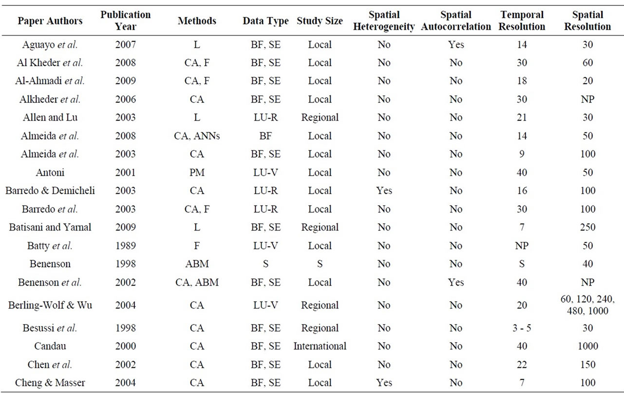

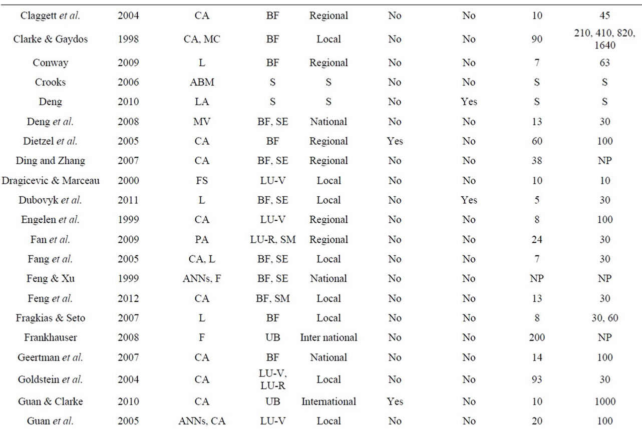


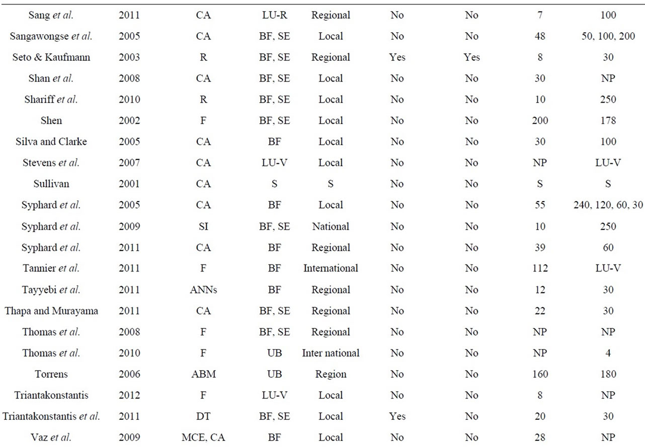
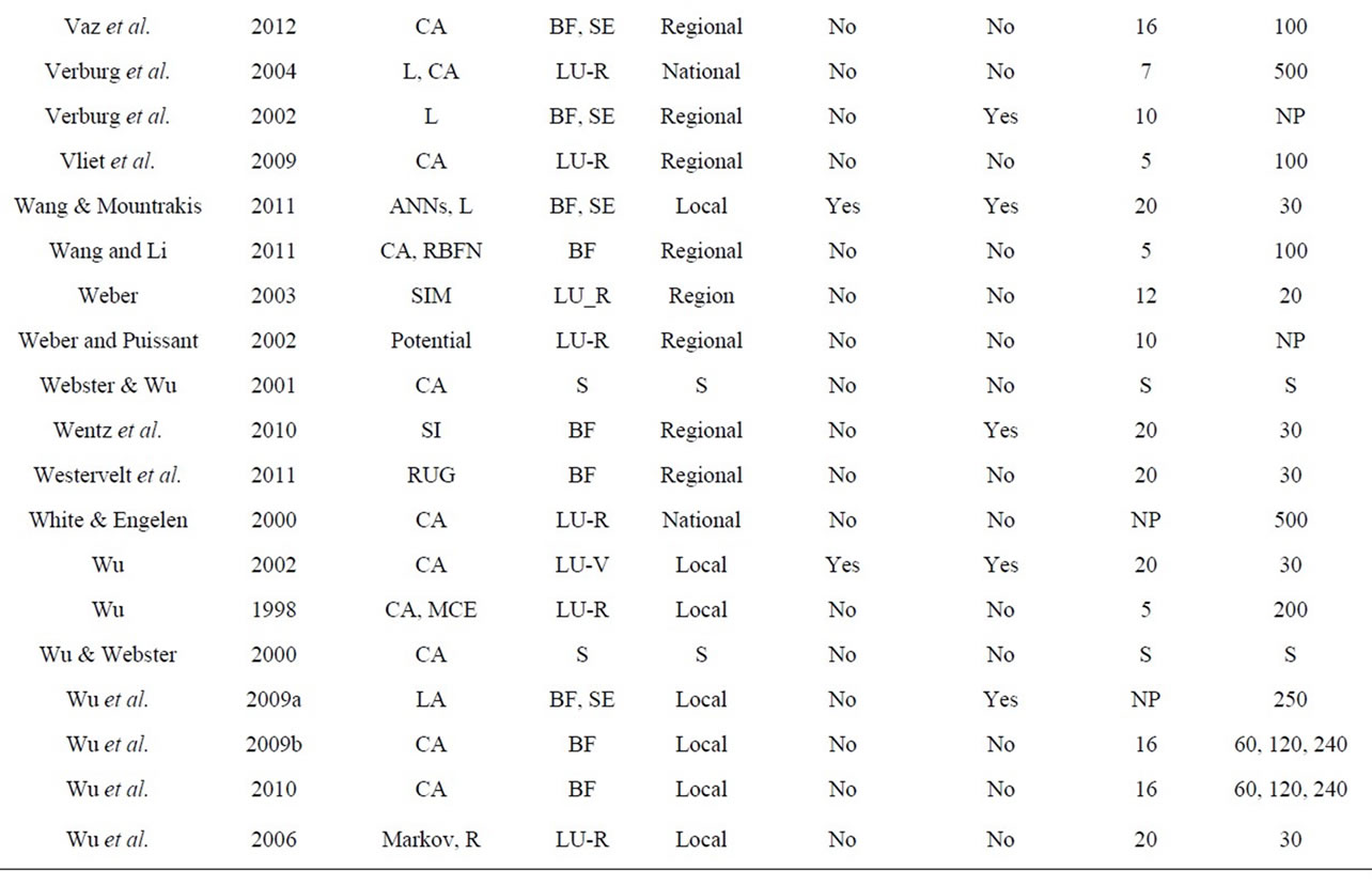
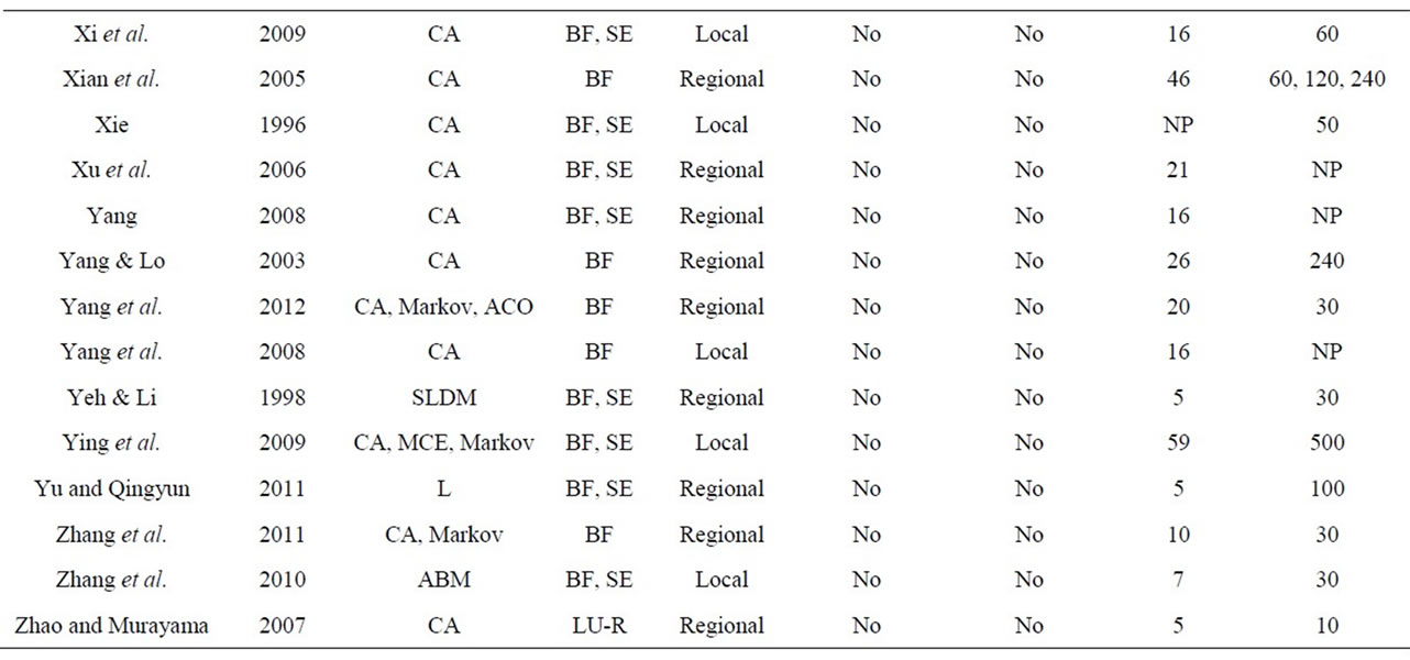
Table S1. Summary table with characteristics of the 156 reviewed manuscripts.
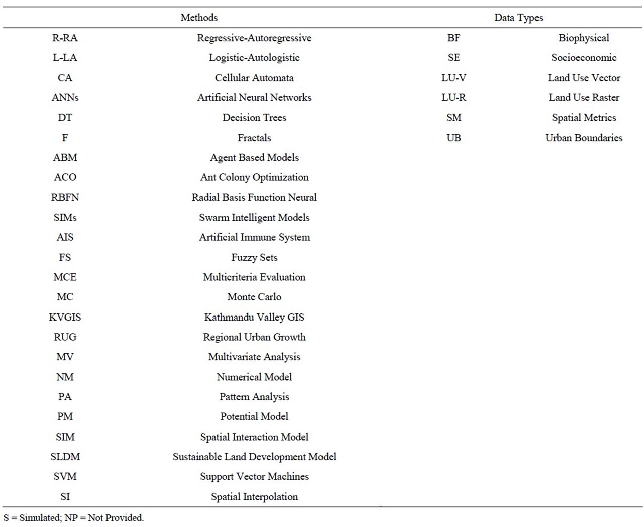
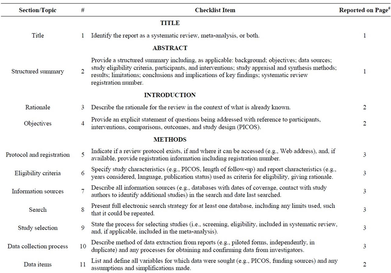
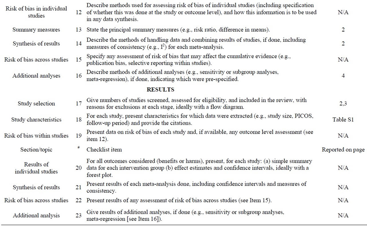

Table S3. PRISMA 2009 checklist regarding the analysis data and manuscript location.
Text S1. Identification of Input Data Sources of UGPMs
In the last decade significant progress has been made in urban data collections, mostly led by governmental agencies and recently followed by private entities. Examples of urban data acquisition include tax offices, transportation departments, utility companies, and emergency management departments [1]. Despite this recent information explosion, collected data may not satisfy urban modeling requirements related for example to spatial and temporal accuracy [2]. In addition, geographical isolation of most collecting efforts makes it challenging to compile data from multiple sites to statistically strengthen confidence on obtained results. Furthermore, the temporal extent of data is constrained, with data from older periods often aggregated at coarser scales.
Data used as input variables in UGPMs are mainly acquired by remotely sensed data and field/sampled data. Each of these sources is discussed in detail in the following subsections.
Remotely Sensed Based Data
Remotely sensed data derived from satellite images and aerial photographs can significantly lower acquisition costs while allowing for broader spatial coverage. An image forms a permanent record that could be revisited at a later time for further information extraction. Even though the United States offers the longest temporal record of remotely sensed data for civilian applications (Landsat series), data collections from other countries have started to offer comparable or improved capabilities, especially for recent data. In addition, several private companies have launched satellite sensors providing costly data but of significantly better spatial resolution, in some cases offering pixel sizes smaller than 1 m.
One of the uses of remotely sensed imagery is the automatic creation of land cover maps. Of particular interest to UGPMs, several remote sensing approaches have been proposed for urban monitoring [3] using methods such as multivariate regression [4,5], spectral mixture analysis [6,7], and machine learning models [8,9]. Even though the majority of these algorithms may reach high classification accuracy, a typical problem is that this accuracy is not spatially distributed in a uniform manner (as shown in [10]) which may generate substantial errors in UGPM calibration.
Landscape topography is another important factor in urban growth. Digital elevation models (DEMs) are derived from stereoscopic analysis of remotely sensed data providing information on elevation, slope, aspect and orientation of the land surface. Because terrain does not change rapidly, DEMs are typically updated every 5 to 10 years and in many UGPMs are assumed to remain constant over time.
In addition to satellite imagery, aerial photographs have been available for more than a century and therefore may extend significantly the temporal coverage of UGPM data, especially if combined with satellite images [11]. Different spatial resolutions along with geometric and radiometric distortions make the integration of aerial photographs with satellite images cumbersome.
Visual interpretation is often implemented to produce a plethora of UGPM inputs. For example, the city of Denver, Colorado obtains its parcel data from visual interpretation of panchromatic aerial photography in order to build a billing system for the wastewater service charge [12]. In the UK, Ordnance Survey produces cadastral data for the entire country, using remote sensed data with ground verification. Numerous transportation departments update their road network vectors, an important urbanization indicator, using remotely sensed data and manual digitizing.
Further spatial processing often takes place on information extracted from remotely sensed data. Typical GIS functions indicating proximity to feature (e.g. distance to nearest road) or feature density (e.g. road density) create high value UGPM inputs [13]. In addition, direct analysis of urban patterns using spatial metrics such as patch size, patch density, edge density, contagion index and fractal dimension have been used as independent variables in UGPMs [14-20].
Satellite images can be also used to derive some useful UGPM inputs expressing socioeconomic data, such as population estimation and life quality indicators (e.g. house value, median family income, average rent) [21,22]. These data can be as accurate as traditional census methods if calibration in situ takes place. Another example of population distribution is LandScan. Produced by Oak Ridge National Laboratory, LandScan is using GIS and Remote Sensing to create a global population distribution with approximate pixel size 1 Km.
Field and Sampling Based Data
Field and sampling based data acquire the precise location of specific points, i.e., coordinates, where GPS receivers can play an important role. The requirements for the types of data as well as their accuracy are different from one study to another, because they are based on the general philosophy of each study. The researcher will decide the kind of data and their accuracy according to expert knowledge and experience of the study area. Moreover, each study requires different spatial and temporal resolutions. For example, different spatial dimensions could be applied in local, regional, national or international levels.
Field surveys help establish a relationship between remote sensing data and the real (ground) environment. Ground data can provide a first-hand view of urban development, useful for understanding urban growth dynamics. The ground control testing corrects the remotely sensed imagery in positions where there is no clear pixel information, e.g. land use boundaries, where spectral mixing is occurring [23].
The classification of built areas requires field-based data. For example, from a field survey, residential and non-residential built areas can be easily discriminated into the following categories: individual houses, buildings, estate housing (residential) and facilities, public buildings, industrial and commercial units (non-residential) [24]. Moreover, some other data can be incorporated to discriminate residential areas such as single-familymulti-family residential [25] and high density-medium density residential, hotel-motel-resort and large lot-small lot residential [26]. [27] acknowledges the importance of human use in land use changing and selected the following field-based data for analyzing urban growth: 1) population density, 2) gross value of industrial output, 3) gross value of agricultural output and d) gross domestic production. Variables related to technology, political and economic institutions as well as cultural values are difficult to include in these analyses because of the complexity of the statistical methods [28].
Field-based data can also provide information about economic activity leading to sprawl [28]. For example, development of service centers such as shopping centers, cafeterias, and bars along a road could become an attracttion point for urban development. Therefore, field-based data becomes valuable information for urban planners and decision makers, once they can visualize such types of growth patterns.
Census and other types of data can be collected by government and other local planning agencies [29,30]. For example, the US Census Bureau provides census and survey data, the most common of which is the population census of the US, called the decennial census, which is conducted every 10 years from each household. Decennial census collects data about income, education, homeownership etc. Additionally, the American Community Survey produces population and housing data every year instead of every ten years. Economic census data of 2007 are available concerning business activities in industries and communities across US; data useful not only for policy planners but also for businesses in order to decide for example a new factory or office location. Annual economic surveys are conducted covering annually, quarterly and monthly time periods for various economy sectors [31]. Moreover, some other census data are also available from US Census Bureau such as statistics about governmental activities, demographic, social, economic and housing characteristic of US population, business and industries. The above census data are collected in different spatial scales: census tract, census block and block groups. Census block is the smallest geographic area, while a block group is a combination of census blocks and a subdivision of a census tract. Census tracts are subdivisions contained within counties. Generally, census data are usually limited in their temporal resolution and consistency, as well as they described by restricted availability in many areas, especially outside developed countries [2].
REFERENCES FOR TEXT S1
- American Planning Association. http://www.planning.org/
- M. Herold, H. Couclelis and K. C. Clarke, “The Role of Spatial Metrics in the Analysis and Modeling of Urban Land Use Change,” Computer, Environment and Urban Systems, Vol. 29, No. 4, 2005, pp. 369-399. doi:10.1016/j.compenvurbsys.2003.12.001
- Q. Weng, “Remote Sensing of Impervious Surfaces,” CRC Press, Boca Raton, 2007, 454 pp. doi:10.1201/9781420043754
- M. Bauer, B. Loeffelholz and B. Wilson, “Estimation, Mapping and Change Analysis of Impervious Surface Area by Landsat Remote Sensing,” Proceedings of Pecora 16 Conference, ASPRS Annual Conference, 23-27 October 2005, Sioux Falls, 9 pp.
- X. Yang, “Estimating Landscape Imperviousness Index from Satellite Imagery,” IEEE Geoscience and Remote Sensing Letters, Vol. 3, No. 1, 2006, pp. 6-9. doi:10.1109/LGRS.2005.853929
- C. Wu and A. T. Murray, “Estimating Impervious Surface Distribution by Spectral Mixture Analysis,” Remote Sensing of Environment, Vol. 84, No. 4, 2003, pp. 493-505. doi:10.1016/S0034-4257(02)00136-0
- J. Franke, D. A. Roberts, K. Halligan and G. Menz, “Hierarchical Multiple Endmember Spectral Mixture Analysis (MESMA) of Hyperspectral Imagery for Urban Environments,” Remote Sensing of Environment, Vol. 113, No. 8, 2009, pp. 1712-1723. doi:10.1016/j.rse.2009.03.018
- T. Esch, V. Himmler, G. Schorcht, M. Thiel and T. Wehrmann, “Large-Area Assessment of Impervious Surface Based on Integrated Analysis of Single-Date Landsat-7 Images and Geospatial Vector Data,” Remote Sensing of Environment, Vol. 113, No. 8, 2009, pp. 1678-1690. doi:10.1016/j.rse.2009.03.012
- L. Luo and G. Mountrakis, “Integrating Intermediate Inputs from Partially Classified Images within a Hybrid Classification Framework: An Impervious Surface Estimation Example,” Remote Sensing of Environment, Vol. 114, No. 6, 2010, pp. 1220-1229. doi:10.1016/j.rse.2010.01.008
- G. Mountrakis, R. Watts, L. Luo and J. Wang, “Developing Collaborative Classifiers Using an Expert-Based Model,” Photogrammetric Engineering and Remote Sensing, Vol. 75, No. 7, 2009, pp. 831-844.
- C. Agarwal, G. M. Green, J. M. Grove, T. P. Evans and C. M. Schweik, “A Review and Assessment of Land-Use Change Models: Dynamics of Space, Time, and Human Choice,” Apollo the International Magazine of Art and Antiques, Vol. 1, No. 1, 2002, 61 pp.
- H. Kienegger, “Assessment of a Wastewater Service Charge by Integrating Aerial Photography and GIS,” Photogrammetric Engineering and Remote Sensing, Vol. 58, No. 11, 1992, pp. 1601-1606.
- J. Wang and G. Mountrakis, “Developing a Multi-Network Urbanization Model: A Case Study of Urban Growth in Denver, Colorado,” International Journal of Geographical Information Science, Vol. 25, No. 2, 2011, pp. 229-253. doi:10.1080/13658810903473213
- M. Herold, H. Couclelis and K. C. Clarke, “The Role of Spatial Metrics in the Analysis and Modeling of Urban Land Use Change,” Computer, Environment and Urban Systems, Vol. 29, No. 4, 2005, pp. 369-399. doi:10.1016/j.compenvurbsys.2003.12.001
- M. Herold, X. Liu and K. Clarke, “Spatial Metrics and Image Texture for Mapping Urban Land Use,” Photogrammetric Engineering and Remote Sensing, Vol. 69, No. 9, 2003, pp. 991-1001.
- X. Li and A. G. Yeh, “Analyzing Spatial Restructuring of Land Use Patterns in a Fast Growing Region Using Remote Sensing and GIS,” Landscape Urban Planning, Vol. 69, No. 4, 2004, pp. 335-354. doi:10.1016/j.landurbplan.2003.10.033
- J. S. Deng, K. Wang, Y. Hong and J. G. Qi, “SpatioTemporal Dynamics and Evolution of Land Use Change and Landscape Pattern in Response to Rapid Urbanization,” Landscape Urban Planning, Vol. 92, No. 3-4, 2009, pp. 187-198. doi:10.1016/j.landurbplan.2009.05.001
- M. Herold, J. Scepan and K. C. Clarke, “The Use of Remote Sensing and Landscape Metrics to Describe Structures and Changes in Urban Land Uses,” Environment and Planning A, Vol. 34, No. 8, 2002, pp. 1443-1458. doi:10.1068/a3496
- Porter-Bolland, E. A. Ellis and H. L. Gholz, “Land Use Dynamics and Landscape History in la Montaña, Campeche, Mexico,” Landscape and Urban Planning, Vol. 82, No. 4, 2007, pp. 198-207. doi:10.1016/j.landurbplan.2007.02.008
- K. McGarigal, S. Tagil and S. Cushman, “Surface Metrics: An Alternative to Patch Metrics for the Quantification of Landscape Structure,” Landscape Ecology, Vol. 24, No. 3, 2009, pp. 433-450. doi:10.1007/s10980-009-9327-y
- C. Lo, “Automated Population and Dwelling Unit Estimation from High-Resolution Satellite Images: A GIS Approach,” International Journal of Remote Sensing, Vol. 16, No. 1, 1995, pp. 17-34. doi:10.1080/01431169508954369
- M. I. Avery and R. Haines-Young, “Population Estimates for the Dunlin Calidris Alpina Derived from Remotely Sensed Satellite Imagery of the Flow Country of Northern Scotland,” Nature, Vol. 344, No. 6269, 1990, pp. 860-862. doi:10.1038/344860a0
- X. Yang, “Satellite monitoring of urban spatial growth in the Atlanta metropolitan area,” Photogrammetric Engineering and Remote Sensing, Vol. 68, No. 7, 2002, pp. 725-734.
- J. Antoni, “Urban Sprawl Modelling: A Methodological Approach,” Cybergeo: European Journal of Geography, 12th European Colloquium on Quantitative and Theoretical Geography, St-Valéry-en-Caux, 7-11 September 2001. doi:10.4000/cybergeo.4188
- E. G. Irwin, N. E. Bockstael and H. J. Cho, “Measuring and Modeling Urban Sprawl: Data, Scale and Spatial Dependencies,” Urban Economics Sessions, 53rd Annual North American Regional Science Association Meetings of the Regional Science Association International, Toronto, 16-18 November 2006, 35 pp.
- M. Luck and J. Wu, “A Gradient Analysis of Urban Landscape Pattern: A Case Study from the Phoenix Metropolitan Region, Arizona, USA,” Landscape Ecology, Vol. 17, No. 4, 2002, pp. 327-339. doi:10.1023/A:1020512723753
- Q. Weng, “Linking Socioeconomic Drivers to Urban Growth to Environmental Effects: A Modeling Approach with GIS and Remote Sensing,” 4th International Conference on Integrating GIS and Environmental Modeling (GIS/EM4): Problems, Prospects and Research Needs, Banff, 2-8 September 2000, 12 pp.
- H. Sudhira, T. Ramachandra, K. Raj and K. Jagadish, “Urban Growth Analysis Using Spatial and Temporal data,” Journal of the Indian Society of Remote Sensing, Vol. 31, No. 4, 2003, pp. 299-311. doi:10.1007/BF03007350
- K. C. Seto and R. K. Kaufmann, “Modeling the Drivers of Urban Land Use Change in the Pearl River Delta, China: Integrating Remote Sensing with Socioeconomic Data,” Land Economics, Vol. 79, No. 1, 2003, pp. 106- 121. doi:10.2307/3147108
- N. Krieger, “Overcoming the Absence of Socioeconomic Data in Medical Records: Validation and Application of a Census-Based Methodology,” American Journal of Public Health, Vol. 82, No. 5, 1992, pp. 703-710. doi:10.2105/AJPH.82.5.703
- US Census Bureau. http://www.census.gov/