Natural Science
Vol.4 No.8(2012), Article ID:21999,12 pages DOI:10.4236/ns.2012.48076
Coupled maps serving the exchange processes on the environmental interfaces regarded as complex systems
![]()
1Faculty of Agriculture, University of Novi Sad, Novi Sad, Serbia; *Corresponding Author: guto@polj.uns.ac.rs
2Department of Mathematics and Informatics, Faculty of Sciences, University of Novi Sad, Novi Sad, Serbia
3Department of Physics, Faculty of Sciences, University of Novi Sad, Novi Sad, Serbia
Received 28 May 2012; revised 30 June 2012; accepted 14 July 2012
Keywords: Coupled maps; Environmental interface; Diffusive coupling; Internal coupling; Map with diffusive coupling; Map with internal affinity; Category Theory; Formal Concept Analysis; Chaos; Complexity; Logistic equation; Cross sample entropy; Permutation entropy
ABSTRACT
We have defined the environmental interface through the exchange processes between media forming this interface. Considering the environmental interface as a complex system we elaborated the advanced mathematical tools for its modelling. We have suggested two coupled maps serving the exchange processes on the environmental interfaces spatially ranged from cellular to planetary level, i.e. 1) the map with diffusive coupling for energy exchange simulation and 2) the map with affinity, which is suitable for matter exchange processes at the cellular level. We have performed the dynamical analysis of the coupled maps using the Lyapunov exponent, cross sample as well as the permutation entropy in dependence on different map parameters. Finally, we discussed the map with affinity, which shows some features making it a promising toll in simulation of exchange processes on the environmental interface at the cellular level.
1. INTRODUCTION
Complex systems science has contributed to our understanding of environmental issues in many areas from small to large temporal and spatial scales (from the cell behavior to global climate and its change). Environmental systems by themselves are both complicated and complex. Complicated, in that many agents act upon them; complex, in that there are feedback loops connecting the state of the system back to the agents, and connecting the actions of the agents to one another. Complex systems have complex dynamics usually characterized by so-called tipping points, abrupt changes in the state of the system caused by seemingly gradual change in its drivers [1]. For example, a climate tipping point is a somewhat ill-defined concept of a point when global climate changes from one stable state to another stable state. After the tipping point has been passed, a transition to a new state occurs. Many scientists now use the power of computer models to advance their subjects. But there is a choice: to simplify complex systems or to include more detail [2]. Further advances in these areas will be necessary before complex systems science can be widely applied to understand the dynamics of environmental systems. In this paper and forthcoming ones we will consider environmental interfaces as complex systems through their main features.
There are many existing researchers that deal with specific aspects of the environmental interface (for example, see references listed above). However, in this paper we rather made an introductory step in establishing the strategy for: 1) modeling of the processes in whole and 2) understanding the functional time of the exchange processes on the environmental interfaces, using new mathematical tools.
1.1. Definition of Environmental Interface
Technically speaking the interface is a point at which independent systems or components meet and act or communicate with each other. Interfaces can exist between system elements and they can also exist between a system element and the system environment when we speak about environmental interface. It can be specifically defined depending on the science where it is used (ecology [3], ecological economy [4], social sciences [5], programming languages and simulation support systems [6], etc.). We define the environmental interface as an interface between two abiotic or biotic environments that are in relative motion and exchange energy, matter and information through physical, biological and chemical processes, fluctuating temporally and spatially regardless of the space and time scale. It is slightly different from its formulation in [7,8]. This definition broadly covers the unavoidable multidisciplinary approach in environmental sciences and also includes the traditional approaches in environmental modeling. For example, such interfaces can be 1) placed in between different environments and 2) extended from micro to planetary scales. Through these interfaces environments exchange energy, matter and information (Figure 1). For example, those processes are: a) ions exchange in metals in unrelaxed configuration of ions and metal cores [9]; b) intercellular exchange of biochemical substances [10]; c) exchange of air volumes in a macroscale of urban conditions [11]; d) periodic migrations between populations [12]; e) heat exchange in Earth’s interior consisting of central core, a mantle surrounding the core and lithosphere; f) energy exchange between solid matter and gas in natural conditions [13] and g) information exchange in a specific environment model combined with the environment interface describing their interactions [14]. The interactions between parts of the complex environmental interface systems are nonlinear, while their interactions with the surrounding environments are noisy that is mathematically well elaborated in [8,15-19], among others.
1.2. Intention of the Paper and Further Plans
The intention of this paper is to be an introductory step in creation of the strategy in modeling the processes on environmental interfaces. It is done trough the following steps: 1) Definition of environmental interface (Subsection 1.1); 2) A concise elaboration of the fundamental tools in environmental interface systems modeling (Section 2) through description of the modeling architecture, use of Category Theory, Mathematical Theory of General Systems and Formal Concept Analysis in Subsections 2.1, 2.2 and 2.3 respectively and 3) description of the two coupled maps, which serve exchange processes on the environmental interface (Subsection 3.1) and numerical simulations with maps of exchange processes on the environmental interface (Subsection 3.2). In papers that would follow we will continue with elaboration of the 1) model of evolvable environmental interfaces and 2) model of forming the functional time of the exchange
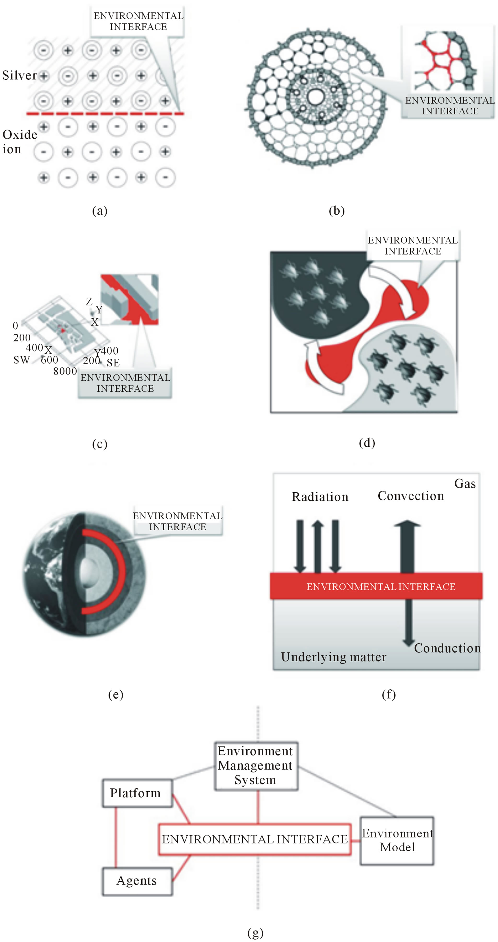
Figure 1. Examples of environmental interfaces: (a) Ions exchange in metals [9]; (b) Intercellular exchange of biochemical substances [10]; (c) Exchange of air volumes in urban conditions [11]; (d) Migration of insects [12]; (e) Heat exchange in Earth’s interior consisting of central core, a mantle surrounding the core and lithosphere; (f) Energy exchange between solid matter and gas in natural conditions [13] and (g) Information exchange in a specific environment model combined with the environment interface describing their interactions [14].
processes on the environmental interfaces.
2. FUNDAMENTAL TOOLS IN ENVIRONMENTAL INTERFACE SYSTEMS MODELLING
The environmental interfaces are formed in a space that is rich with complex systems. Each system, as an open one, interacts in a coherent way, producing new structures and building cohesion and new structural boundaries. It undergoes emergence and self-organization. In modeling the complex environmental interface systems, except the traditional mathematical, are often used the new mathematical tools like Category Theory (originally proposed by Rosen [20]), Mathematical Theory of General Systems [21] and Formal Concept Analysis (FCA) [22,23].
2.1. Modeling Architecture
Modelers of environmental interface systems in numerically oriented studies base their calculations on mathematical models for the simulation and prediction of different processes, which are exclusively nonlinear in describing relevant environmental quantities [20]. A theoretical description of any environmental interface system includes at least two important aspects. First, one should construct a concrete mathematical model of both the admissible states of the system and the transitions between these states. Second, one should establish the rules of selecting among the many theoretically admissible states of the system only those states that are realized in nature under the given external conditions [24].
In modeling community dealing with complex systems, Rosen’s diagram ([20] see Figure 2.3.1 p. 74, which represents the modeling relation) is a recognizable guide. Figure 2 is slightly modified Rosen’s diagram and schematically depicts a modelling relation when a natural system (N) and a formal system (F) are given. As above, two arrows represent the respective entailment structures; inference in formalism (F) and causality in a natural system (N). Now, the two established dictionaries provide encoding the phenomena of N into the propositions of F

Figure 2. Schematic diagram representing both 1) the comparison of two formalisms F1 and F2 and 2) modeling relation when we have given a natural system N and a formal system F [7]. Here, 1 represents causal entailment within the natural system (N); 2 represents encoding, where the observer’s propositions about N are used as hypotheses in constructing formal system (F); 3 is the generation of theorems in F, which function as a model of N; and 4 is decoding, where the theorems of F are applied back to N in the form of predictions.
and another for decoding the propositions of F back to the phenomena in N. As mentioned above, there are two paths in diagram (1) and (2) + (3) + (4). According to [20] the first of them (the path (1)) represents the causal entailment within N (what an observer will see by simply sitting and watching what is happening). The arrow (2) encodes the phenomena in N into the propositions in F. In this route we must use these propositions as hypotheses based on which the inferential machinery of the formal system F may operate (denoted by the arrow (3)); it generates theorems in F, entailed precisely by the encoded hypotheses. Finally, we have to decode these theorems back into the phenomena of N, via the arrow (4). At this point, the theorems become predictions about N. Then the formal system F is called a model of the natural system N if we always get the same answer regardless of the fact whether we follow path (1) or path (2) + (3) + (4). The process of modelling complex systems is a very comprehensive one. A system is to be treated as a complex structure, as for instance in Peter Checkland’s definition: A system is a model of a whole entity; when applied to human, the model is characterised fundamentally in terms of hierarchical structure, emergent properties, communication and control ([25], p. 318). The major components of complexity are openness and freeness, but the distinctive characteristic is “natural activity” like self-organisation, and still of great importance as intraactivity but now joined by the phenomena of anticipation [26] and interactivity between systems to be found in global interoperability. The transition from connectivity to activity involves a type change and therefore requires formal system with an inbuilt facility to cross between the levels. Thus, intraconnectivity between the components cannot give rise to interactivity between those components without some non-local integrity coming into play [27]. The non-locality is a principle that is, among some others, specific for a certain object area such as the inorganic, living or human realm. This principle means certain interaction between the elements of the system that is treated as the transmission of information at infinite speed (see, for instance, [28]).
2.2. Use of Category Theory
Category Theory recommended by Rosen [20] as a modern tool for complex (and living) systems is found to have a formal expressive power for exploring the fundamental non-local concept of adjointness needed to understand complex systems. The arrow of Category Theory does not only have a formal meaning. According to [27] it formalizes the principle of constancy (originally introduced by Heraclites and Parmenides) that is provided by a common source and target. Such an arrow refers to the situation in which a source and target are indistinguishable. In a defined system, the collection of entities can be identified as objects, while operations between them are defined by arrows. Figure 3 shows that there may be many possible arrows between objects. However, Category Theory holds that a unique limiting arrow may exist for all of these possible arrows that represent the resulting intraconnectivity of a local system. There is an order between the two entities established by the directions of arrows [29]. This means that the arrow limit between two entities is also a limit of all possible paths. Because of the existence of limits and all possible connectivity, this is classified by axiomatic categories as a Cartesian closed category. Moving up one level, there is a grand limiting arrow for all of the aforementioned limits, existing as an identity functor characterizing the type and therefore the system as a category (Figure 4). A system as a category may then be drawn as a circular arrow, which is the identity functor that identifies the type of a system [27,29]. Therefore, the system can be represented as an arrow, i.e., a process in which the internal arrows are simply the components of one arrow. This then leads to interconnectivity between the systems. Also, the functor between two categories is conceptually the same as internal arrows between the arrows above. Within the framework of this theory, it is possible to repeat the abstraction to one level higher, to so called natural transformations. This level is the level of interactivity. It is important to note that the self-organization of a Category Theory-system (intra-activity) arises when the category-system pair is indistinguishable. Finally, Category Theory is a very useful tool when we meet difficult problems in some areas of mathematics, ecology, physics, computer sciences, biological nano-engineering and the self-organization of cell function in living systems [30], among many others. They can be translated into (easier) problems in other areas (e.g., by using functors, which map one category to another).
2.3. Use of Mathematical Theory of General Systems
Following Mesarovic’s Mathematical Theory of General Systems [21], if we observe interactions of agents with their surrounding environment, such a system can be defined as a set of interacting objects 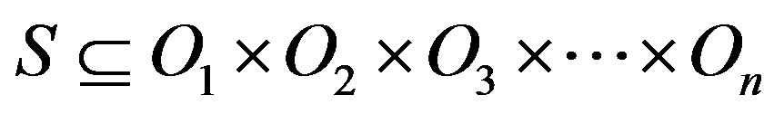 . If we denote the population of agents under consideration as
 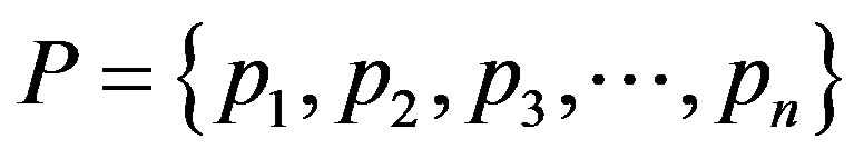 and a set of external influences as
 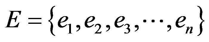 (these influences can be either other agents or extra-systemic influences), then the state of such formed systems at any particular moment in time can be defined as the Cartesian product
 . Because our system is a dynamical network of interactions where at each moment the hierarchical status of network elements can vary significantly, we have to define state of the population P as a mapping
 ,
, . Both e and p are defined as temporal sequences of events such that
  and
and , where T is a set of time points t, I is a set of external stimuli on a particular agent such that at each time system receive stimulus
  and R is a set of responses,
 . Furthermore, both P and E are formal systems. Therefore, the occurrence of p and occurrence of e at some particular time point t are governed not only by mapping
  but also by the internal rules of these systems, which are partially independent.
Thus, it is obvious that changes in an environment induce appropriate responses in agents through the model of coupled input/output pairs. In real systems, the reverse situation is also possible such that some external changes can be influenced by the activity of organisms, but for the sake of simplicity and because it is not directly related to the main topic of this presentation, we will not consider that problem. It is clear that a critical factor in building an evolvable model as described above is choosing the appropriate structure for the mapping . When dealing with models usually developed as prediction tools, it is sufficient to assume the attitude of analyzing a “black box”. Therefore, we can propose a function that should summarize all available experimental data and obtain a set of more or less accurate predictions for various initial conditions. However, in such a case we will neglect the real meaning of the nature of mappings within E and P. Taking a slightly closer look at these relations we can see that a somewhat hidden problem is that of how I is generated from the
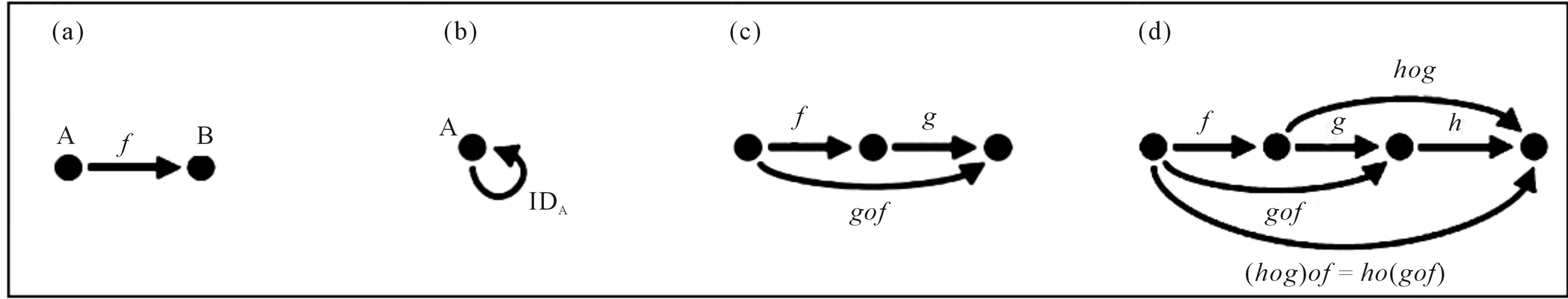
Figure 3. Schematic diagram representing the Category Theory essentials: (a) Morphism (arrows), objects, domain and co-domain; (b) Identity morphism; (c) Composite morphism and (d) Identity composition and associativity.

Figure 4. Schematic diagram representing the functor “action” (dashed line).
wholeness of external changes and what is the connection between generating I with a constitution of corresponding R. Although this connection can be efficiently represented using the FCA [23], its evolvability demands a more advanced formal treatment to be fully comprehended.
3. COUPLED MAPS IN PROCESSES OF EXCHANGE ON THE ENVIRONMENTAL INTERFACE SYSTEMS
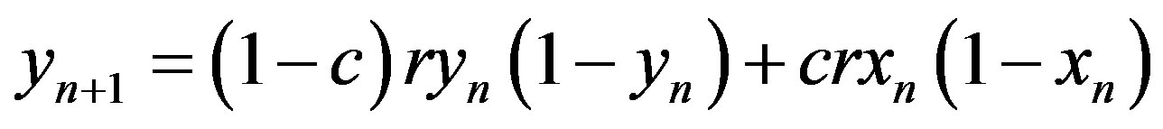
Many physical, biological as well as the environmental interface issues, can be described by the dynamics of coupled maps. In environmental models various non-linear dynamics methods are used (for example, [8,12,31-33]). However, in modeling of exchange energy and matter in environmental interface it is useful to use 1) the diffusive coupling, which describes the energy exchange [8,13] and 2) the mapping with internal affinity, that describes the matter exchange [10]. The map with diffusive coupling (in further text, diffusive map) has the form
 (1a)
(1a)
 , (1b)
where parameter 
 is the so-called logistic parameter, while
  is the coupling parameter. Since the first map is described in [13] and partly in [8] here the second map will be described in more details.
3.1. The Map with Internal Affinity
The map with internal affinity (in further text-map with affinity) can be used for describing the matter exchange in various biological as well as biophysical environmental interfaces. However, here we will consider it through intercellular exchange with the cell membrane as an environmental interface. As it is obvious from the empirical description, we can infer the successfulness of the communication process by monitoring: 1) the number of signaling molecules, both inside and outside of the cell and 2) their mutual influence. The concentration of signaling molecules in an intercellular environment is subject to various environmental influences, and taken alone often can indicate more about state of the environment than about the communication itself. Therefore, we choose to follow the concentration of signaling molecules inside of the cell as the main indicator of the process. In this case, the parameters of the system are 1) the affinity  by which cells perform uptake of signaling molecules (a2), which depends on the number and the state of the appropriate receptors, 2) the concentration c of the signaling molecules in the intercellular environment within the radius of interaction, 3) the intensity of the cellular response (a1)
  and
and  and 4) the influence of other environmental factors, which can interfere with the process of communication. In this case we estimate parameter
  which can be taken collectively for intraand intercellular environments inside of the one variable, indicating the overall disposition of the environment to the communication process.
The time development ( is the number of time steps) of the concentration in cells
  can be expressed as
 , (2a)
 . (2b)
The map,  represents the flow of materials from cell to cell, and
  and
and  are defined by a map that can be approximated by a power map,
  and
and . If
. If  and
and , the interaction is expressed as a nonlinear coupling between two cells. The dynamics of intracellular behavior is expressed as a logistic map (e.g. [34,35]),
 . (3)
. (3)
Because the concentration of the signaling molecules can be regarded as their population for a fixed volume, and because we are focused on the mutual influence of these populations, it is clear that we should use the coupled logistic equations. Instead of considering cell-to-cell coupling of two explicit n-gene oscillators [36], we consider the generalized case of intercellular communication. In this case, the investigation of conditions for which two equations are synchronized and how this synchronization behaves under changes of intraand intercellular environments can give some answers to the question of how functionality in the system is maintained. Therefore, having in mind 1) that cellular events are discrete [37] and 2) using the aforementioned reasoning, we consider systems of difference equations of the form
 , (4)
, (4)
with notation
 (5)
(5)
where  is a vector representing the concentration of the signaling molecules inside of the cell, while
  denotes the stimulative coupling influence of members of the system, which is here restricted only to positive numbers in the interval (0, 1). The starting point
  is determined such that
 . Parameter
  in logistic difference equations determines an overall disposition of the environment to the given population of signaling molecules and exchange processes. The affinity to uptake signaling molecules is indicated by
 . Let us note that we require that the sum of all affinities of cells
  exchanging substances has to satisfy the condition
  or in the case of two cells,
 , i.e.,
 . Because
  is a fixed point (4), in order to ensure that zero is not simultaneously the point of attraction, we define
  as an exponent. Finally,
  represents coupling of two factors: the concentration of the signaling molecules in the intracellular environment and the intensity of response they can provoke. This form is taken because the effect of the same intracellular concentration of signaling molecules can vary greatly with variation of affinity of genetic regulators for that signal, which is further reflected in the ability to synchronize with other cells. Therefore,
  influences both the rate of intracellular synthesis of signaling molecules and the synchronization of the signaling processes between two cells, so the parameter
  (the coupling parameter) is taken to be a part of both
  and
and . However, the relative ratio of these two influences depends on the current model setting. For example, if for both cells,
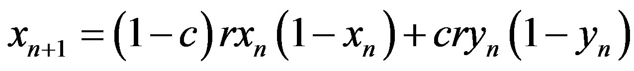
  is strongly influenced by the intracellular concentration of signals that can provoke relatively smaller responses, then the form of equation will be
 , (6a)
 . (6b)
We now analyze our coupled system, given by (6a) and (6b). For  and
and , we have
  . So, for small
 , the dynamic of our investigated system is similar to the dynamic of the following systems obtained by minorization, as follows
 (7)
(7)
and 
 (8)
(8)
If we apply a majorization, the considered system becomes
 (9)
(9)
For all of these systems, it is obvious that they do not depend on the parameter . Because
 , where
  are the components of
  in (8), their dynamics are symmetric to the diagonal
 ,
,  . This symmetry also exists for system (6a)-(6b), if
 .
.
Recalling the aforementioned conditions for ,
,  and
and , we consider only systems (7) and (9) because the behavior of the system (6a)-(6b) comes from the properties of the mentioned ones. It is seen that the systems (7) and (9) consist of uncoupled logistic maps on the interval
  (in (7)) or on the interval
  (in (9)), where
  is the smaller solution of the equation
  i.e.
i.e.
 .(10)
.(10)
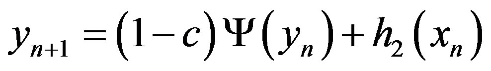
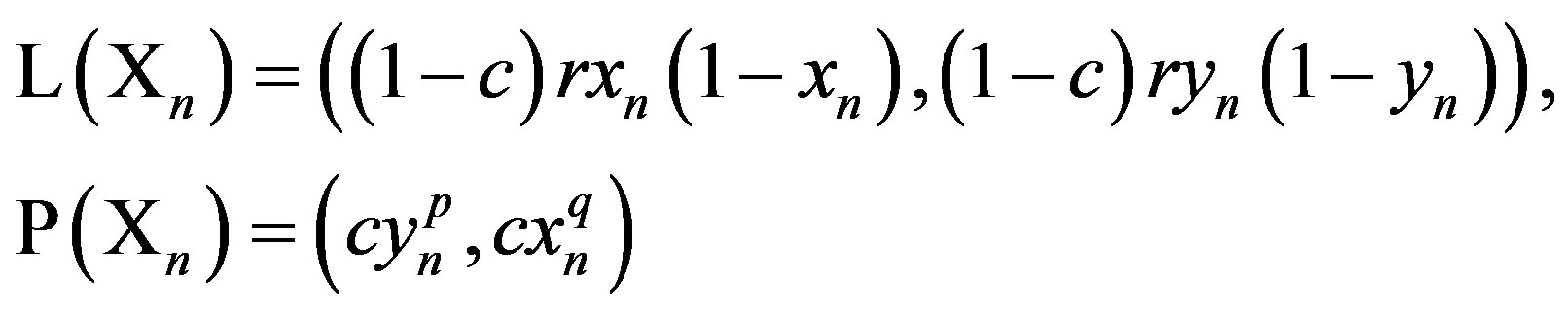
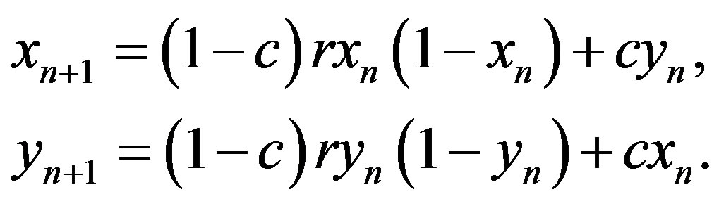
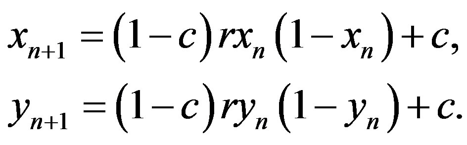
Finally, let us note that the map, which describes exchange processes, can be generalized in the form
 (11a)
(11a)
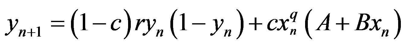 . (11b)
This system we will call map of exchange processes. Specially, for  and
and  we get the diffusive map, while for
  and
and ,
,  we get the map with affinity.
3.2. Numerical Simulations with Maps of Exchange Processes on the Environmental Interface
In the analysis of these coupled maps we will consider three parameters included in the archive of dynamical analysis of coupled maps: 1) the largest Lyapunov exponent, 2) the cross sample entropy (Cross-SampEn) and 3) the permutation entropy (PermEn). We calculate the largest Lyapunov exponent  to see the behaviour of the coupled maps given by Eqs.1a-1b and 6a-6b, as particular cases of Eqs.11a-11b, depending on different values of the coupling parameter
 . Extending the approach in [38,39], we study, for two coupled maps representing biochemical substance exchange between cells, the stability of the fixed point by linearizing Eqs.11a- 11b.
 (12)
(12)
where
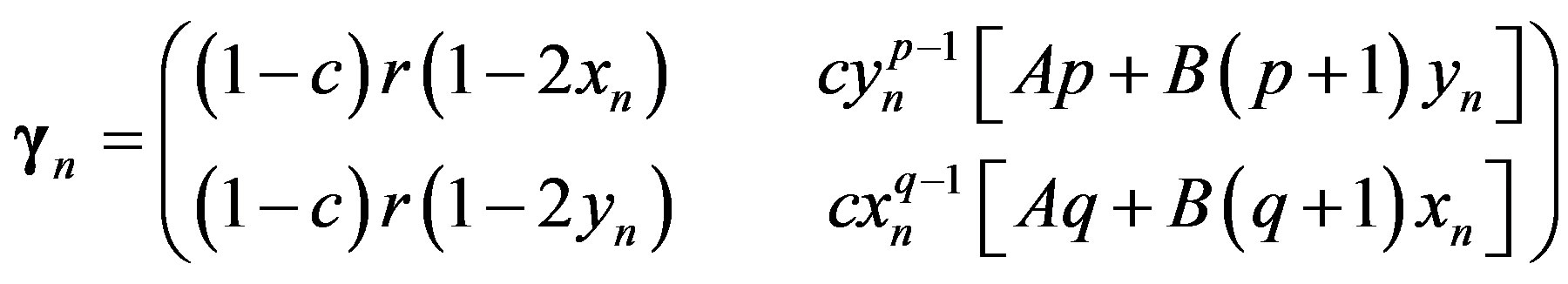 (13)
(13)
is the Jacobian of the system (11) evaluated in  and
and . By iterating Eq.12 one obtains
 (14)
(14)
and thus we get Lyapunov exponent [40], i.e.
 (15)
(15)
Figure 5 depicts Lyapunov exponent for the both coupled maps as a function of 1) coupling parameter ranging from 0 to 1, with the increment of 0.001, and 2) four different values of the logistic parameter
  within the chaotic region or close to it. Each point was obtained by iterating 1000 times from the initial condition to eliminate transient behavior and then averaging over another 600 iterations starting from initial condition
  and
and . From Figure 5(a) it is seen that for period 16 (
 ), the Lyapunov exponent of the diffusive map has either negative values or ones, which are very equal or close to zero on the whole interval of the coupling parameter
 . The Lyapunov exponent for this map has 1) values, when the coupling parameter
  is in the interval
  and 2) the negative values in intervals
  and
and  and the logistic parameter
  takes values that lie in the chaotic region, i.e. a) low chaos (
 ), b) high chaos (
 ) and c) intermittency (
 ), as seen in Figures 5(b)-5(d). Similarly, to the behavior of
 , for period 16, of the map with affinity takes either negative or values close to zero (Figure 5(a)). From Figures 5(b)-5(d) that intervals with positive
  values become broader with sporadic windows with negative values, when values of
  takes greater values in the chaotic region, i.e. for a)
  (
( ), b)
), b)  (
( ) and c) for
  (
( ). Here, we will note a feature of the map with affinity that is related to events on the environmental interface on the cellular level. Namely, the self-organization of proteins is of crucial importance for the functioning of cellular processes. However, this organization often takes place in the presence of strong random fluctuations [41] due to the small number of molecules involved. In particular it remains largely unexplored how fluctuations at cellular scales originate from the interplay of molecular and external noise [42]. This map shows that for small values of coupling parameter
  (concentration) and higher values of the logistic parameter
  chaotic fluctuations prevails while synchronization appear (
 ) with increase of
  (red line in Figures 5(b)-5(d)).
Cross-SampEn measure of asynchrony is a recently introduced technique for comparing two different time series to assess their degree of asynchrony or dissimilarity [43,44]. Let  and
and
 fix input parameters
  and
and
 . Vector sequences:
  and
and  and
and  is the number of data points of time series,
 . For each
  set
set  = (number of
  such that
 ), where
 ranges from 1 to
 , and then
 which is the average value of
 . Similarly we define
and  as
as  = (number of
such that ) and
) and
 which is the average value of
 . Finally, we have
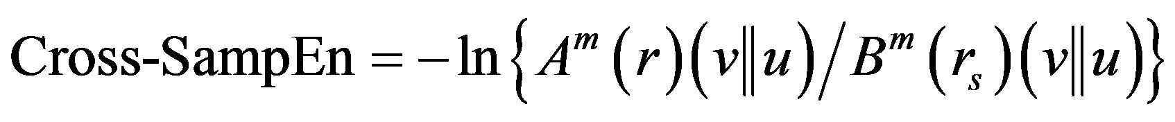 . (16)
We applied Cross-SampEn with  and
and  for
for  and
and  time series, and the same range of parameters
  and
and  for which the Lyapunov exponent is calculated (Figures 5(a), (b)). Figure 6 depicts the CrossSampEn for the diffusive map and map with affinity given by the coupled systems (1) and (6), respectively. From a simple inspection of Figure 6(a) it is seen, that for period 16, the Cross-SampEn of the diffusive map has values close to zero since
  is near to zero on the whole interval of the coupling parameter
 . The CrossSampEn for this map has 1) the values greater than zero, when the coupling parameter
  is in the interval (0.2, 0.8) and 2) the negative values in intervals (0.1, 0.2) and (0.8, 0.9) when the logistic parameter
  takes values from the chaotic region, i.e. a) low chaos, b) high chaos and c) intermittency, as it is seen in Figures 6(b)-(d). The Cross-SampEn, for period 16, the map with affinity dominantly takes values equal to zero (Figure 6(a)), except in the interval
 . Let us note that CrossSampEn is equal to zero for,
  and positive for
 . This is clearly seen from Figures 6(b)-(d) where values of Cross-SampEn follows the Lyapunov exponents in Figures 5(b)-(d) for all values of the logistic parameter
 .
.
Permutation Entropy (PermEn) of order  is de- fined as PermEn
  where the sum runs over all
  permutations
  of order
 . This is the information contained in comparing
  consecutive values
 (a)
(a) (b)
(b) (c)
(c) (d)
(d)
Figure 5. Lyapunov exponent for the diffusive map and map with affinity given by the coupled systems (1) and (6), respectively. Calculations are performed for 1) the four different values of the logistic parameter  within the chaotic region or close to it and 2) all values of the coupling parameter c on the interval [0, 1].
of the time series. Consider a time series . We consider all
  permutations
  of order
  which are considered here as possible order types of
  different numbers. For each
  we determine the relative frequency
  has type
 . This estimates the frequency of
  as good as possible for a finite series of values. To determine
  exactly, we have to assume an infinite time series
  and take the limit for
  in the above formula. This limit exists with probability 1 when the underlying stochastic process fulfills a very weak stationarity condition: for
 , the probability for
  should not depend on
 . Permutation entropy as a natural complexity measure for time series behaves similar as Lyapunov exponents, and is particularly useful in the presence of dynamical or observational noise [45]. With increased model complexity we are less able to manage and understand model behaviour. As a result, the ability of a model to simulate complex dynamics is no more an absolute value in itself, rather a relative one: we need enough complexity to realistically model a process, but not so much that we ourselves can not handle [46]. For example, if we want to model biophysical processes on environmental interfaces we meet
 (a)
(a) (b)
(b)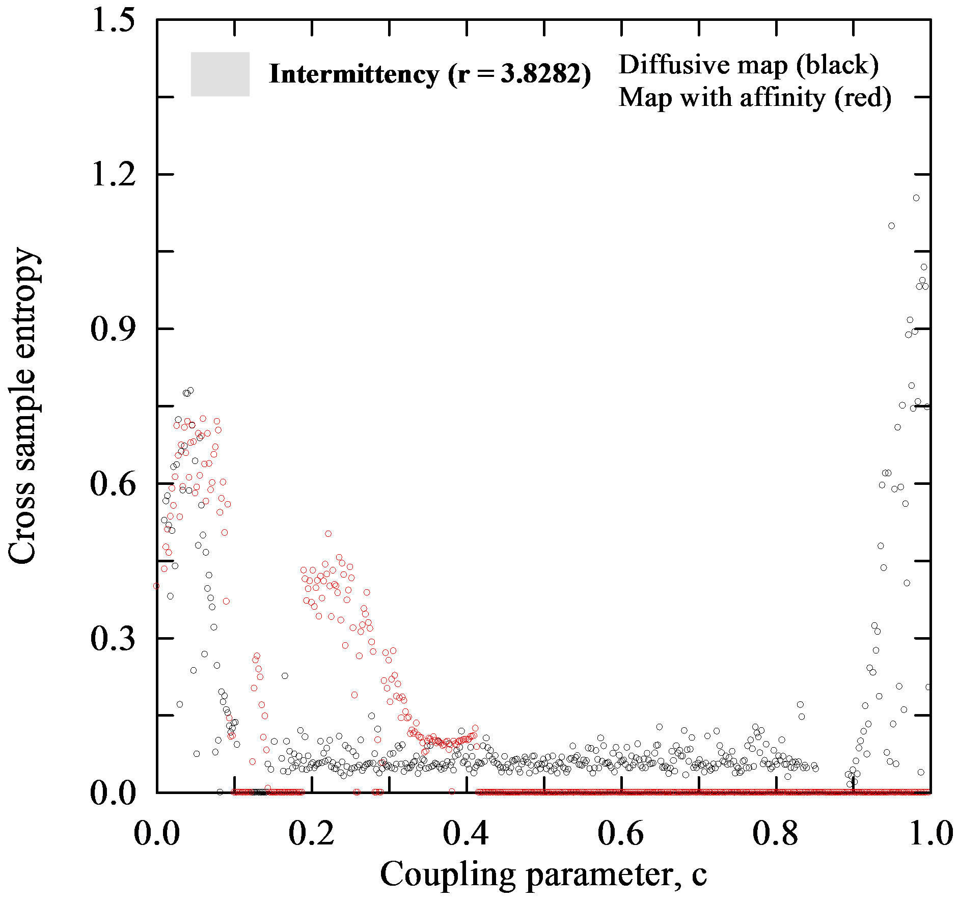 (c)
(c)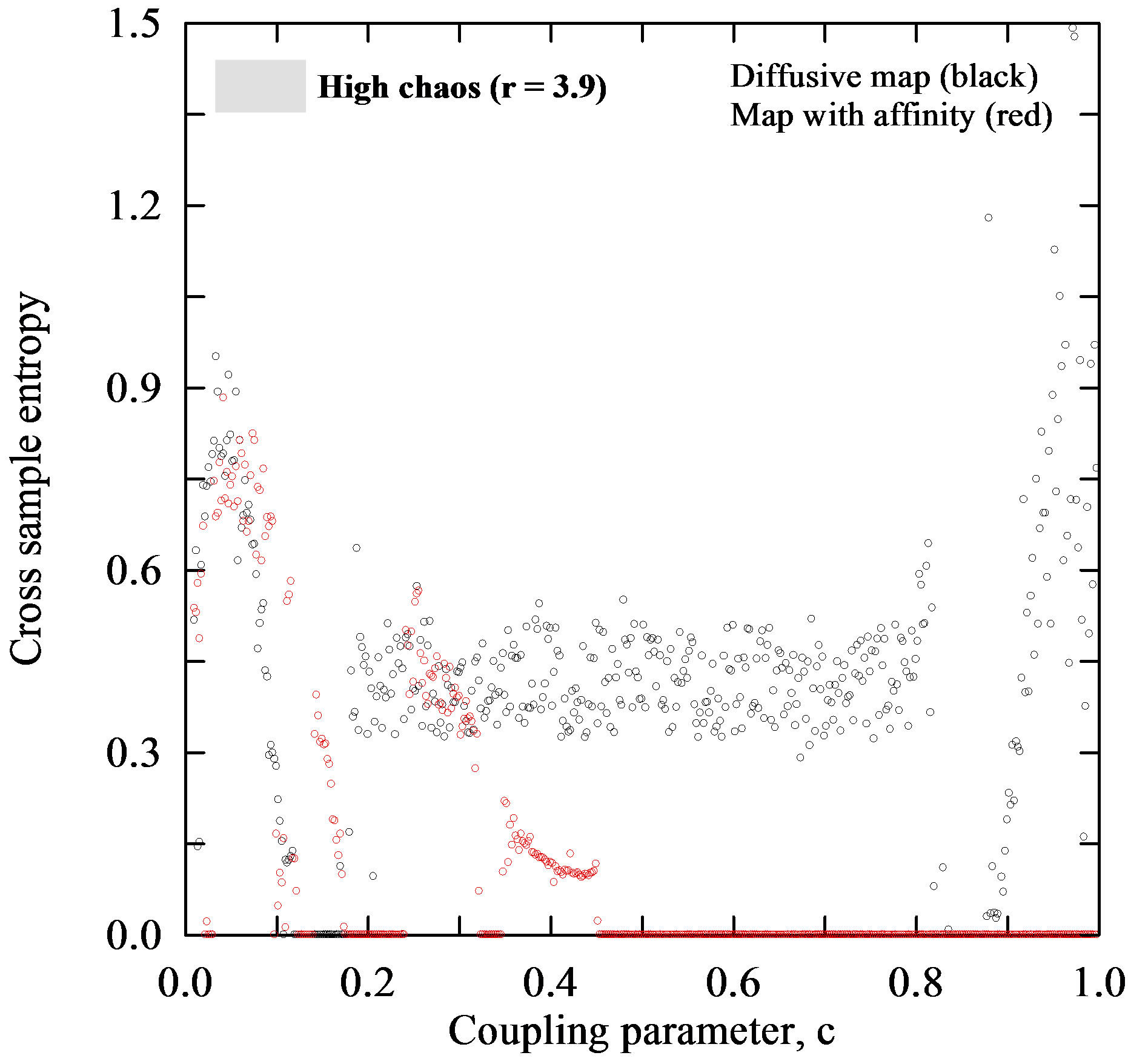 (d)
(d)
Figure 6. Cross sample entropy for the diffusive map and map with affinity given by the coupled systems (1) and (6), respectively. Calculations are performed for 1) the four different values of the logistic parameter  within the chaotic region or close to it and 2) all values of the coupling parameter
  on the interval [0, 1].
a lot of uncertainties in time series of calculated physical quantities. Various measures of complexity were developed to compare time series and distinguish regular (e.g., periodic), chaotic, and random behaviour. The main types of complexity parameters are entropies and the Lyapunov exponent, among others. They are all defined for typical orbits of presumably ergodic dynamical systems, and there are profound relations between these quantities [47]. Figures 7(a)-(d) depict the calculated values of the PermEn versus the coupling parameter , which is periodic for some regions and chaotic for others. It can be also clearly seen some regions of stability for both maps. Let us note that PermEn, as a natural complexity measure for time series, behaves similarly to Lyapunov exponents (Figures 7(a)-(d) vs. 5(a)-(d)).
4. CONCLUSIONS
Our main results in this paper can be summarized as follows. 1) We have defined the environmental interface through exchange energy, matter and information between media forming this interface. 2) Considering environmental interface as a complex system we shortly described the advanced mathematical tools that can be
 (a)
(a) (b)
(b)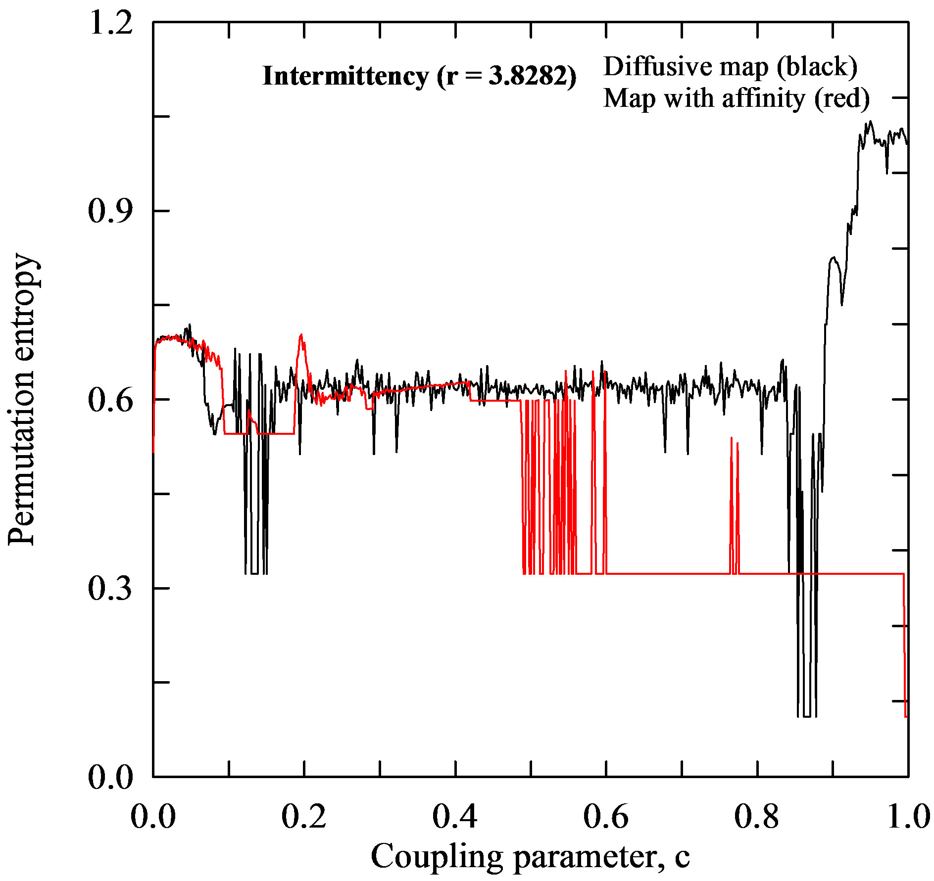 (c)
(c)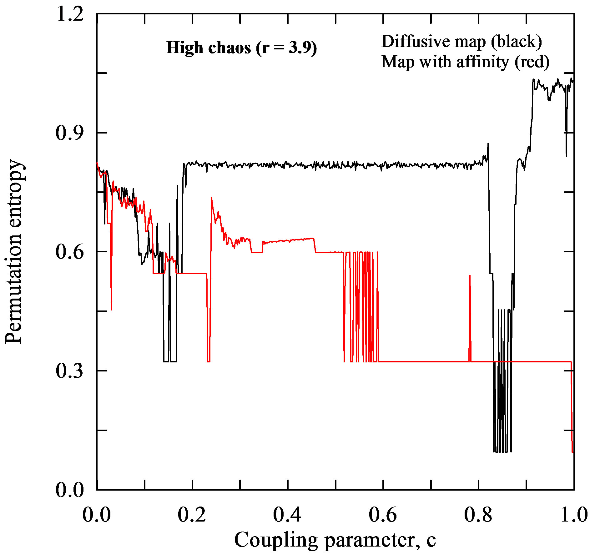 (d)
(d)
Figure 7. Permutation entropy for the diffusive map and map with affinity given by the coupled systems (1) and (6), respectively. Calculations are performed for 1) the four different values of the logistic parameter  within the chaotic region or close to it and 2) all values of the coupling parameter
  on the interval [0, 1].
used in its modelling (Category Theory, Mathematical Theory of General Systems and Formal Concept Analysis). 3) We suggested the two coupled maps serving the exchange processes on the environmental interfaces spatially ranged from cellular to planetary level, i.e. a) the map with affinity, which is suitable for matter exchange processes at cellular level and b) the map with diffusive coupling for energy exchange simulation. 4) For maps (1a)-(1b), representing diffusive coupling and (6a)-(6b), that describes coupling with internal affinity, with controlling parameters ( ) and (
 ), respectively we calculated the largest Lyapunov exponent, sample as well as the permutation entropy. 5) The Lyapunov exponent
  for the diffusive map has 1) positive values, when the coupling parameter
  is in the interval
  and 2) negative values in intervals
  and
and , while logistic parameter
  takes values that lie in the chaotic region, i.e. low chaos (
 ), high chaos (
 ) and intermittency (
 ). For period 16 its values are either negative or very close to zero. 6) Similarly to diffusive map, in the map with affinity, for period 16,
  takes either negative or values close to zero. However, the intervals with positive
  values become broader with sporadic windows with negative values, when
  takes greater values in the chaotic region, i.e.
  (
( ),
), (
( ) and
) and  (
( ). 7) Calculated values of the Cross-SampEn are mostly equal or very close to zero, corresponding to the region where
  is negative, indicating a high level on synchronization between quantities
  and
and . Also, the calculated values of the PermEn, as a natural complexity measure for time series behave similarly as Lyapunov exponents. 8) The map with affinity shows some features, which make it a promising toll in simulation of exchange processes on the environmental interface at cellular level.
5. ACKNOWLEDGEMENTS
This paper was realized as a part of the project “Studying climate change and its influence on the environment: impacts, adaptation and mitigation” (43007) financed by the Ministry of Education and Science of the Republic of Serbia within the framework of integrated and interdisciplinary research for the period 2011-2014. We are appreciated to Miss Ana Firanj for designing the figures.
REFERENCES
- Gladwell, M. (2000) The tipping point: How little things can make a big difference, first edition. Little Brown, London.
- Paola, C. and Leeder, M. (2011) Environmental dynamics: Simplicity versus complexity. Journal name: NatureVolume: , 469, Pages: 38-39. doi:10.1038/469038a
- Sizykh, A.P. (2007) Plant communities of environmental interfaces as a problem of ecology and biogeography. Biollogy Bulletin, 34, 292-296. doi:10.1134/S1062359007030120
- Lehtonen, M. (2004) The environmental-social interface of sustainable development: Capabilities, social capital, institution. Ecological Economics, 49, 199-214. doi:10.1016/j.ecolecon.2004.03.019
- Rasmussen, K. and Arler, F. (2010) Interdisciplinarity at the human-environment interface. Danish Journal of Geography, 110, 37-45.
- Banks, J., Carson, J.S., Nelson, B.L. and Nicol, D.M. (2009) Discrete-event system simulation. Prentice Hall, Upper Saddle River.
- Mihailovic, D.T. and Balaž, I. (2007) An essay about modeling problems of complex systems in environmental fluid mechanics. Idojaras, 111, 209-220.
- Mihailović, D.T., Budinčević, M., Perišić, D. and Balaž, I. (2012) Maps serving the combined coupling for use in environmental models and their behaviour in the presence of dynamical noise. Chaos, Solitons & Fractals, 45, 156- 165. doi:10.1016/j.chaos.2011.11.005
- Duffy, D.M., Harding, J.H. and Stoneham, A.M. (1992) Atomistic modeling of the metal/oxide interface with image interactions. Acta Metallurgica et Materialia, 40, 11-16. doi:10.1016/0956-7151(92)90258-G
- Mihailović, D.T., Budincevic, M., Balaž, I. and Mihailović, A. (2011) Stability of intercellular exchange of biochemical substances affected by variability of environmental parameters. Modern Physics Letters B, 25, 2407-2417. doi:10.1142/S0217984911027431
- Neofytou, P., Venetsanos, A.G., Vlachogiannis, D., Bartzis, J.G. and Scaperdas, A. (2006) CFD simulations of the wind environment around an airport terminal building. Environmental Modelling & Software, 21, 520- 524. doi:10.1016/j.envsoft.2004.08.011
- Lloyd, A.L. (1995) The coupled logistic map: A simple model for effects of spatial heterogeneity on population dynamics. Journal of Theoretical Biology, 173, 217-230. doi:10.1006/jtbi.1995.0058
- Mihailović, D.T., Budinčević, M., Kapor, D., Balaž, I. and Perišić, D. (2011) A numerical study of coupled maps representing energy exchange processes between two environmental interfaces regarded as biophysical complex systems. Natural Science, 1, 75-84.
- Behrens, T.M., Dix, J. and Hindriks, K.V. (2009) Towards an environment interface standard for agent-oriented programming. Technical Report IfI-09-09, Clausthal University of Technology.
- Serletis, A., Shahmoradi, A. and Serletis, D. (2007) Effect of noise on the bifurcation behavior of nonlinear dynamical systems. Chaos, Solitons & Fractals, 33, 914- 921. doi:10.1016/j.chaos.2006.01.046
- Serletis, A., Shahmoradi, A. and Serletis, D. (2007) Effect of noise on estimation Lyapunov exponents from a time series. Chaos, Solitons & Fractals, 32, 883-887. doi:10.1016/j.chaos.2005.11.048
- Serletis, A. and Shahmoradi, A. (2006) Comment on ‘‘Singularity Bifurcations’’ by Yijun He and William A. Barnett. Journal of Macroeconomics, 28, 23-26. doi:10.1016/j.jmacro.2005.10.002
- Savi, M.A. (2007) Effects of randomness on chaos and order of coupled maps. Physical Letters A, 364, 389-395. doi:10.1016/j.physleta.2006.11.095
- Liu, Z. and Ma, W. (2005) Noise induced destruction of zero Lyapunov exponent in coupled chaotic systems. Physical Letters A, 343, 300-305. doi:10.1016/j.physleta.2005.06.044
- Rosen R. (1991) Life itself, a comprehensive inquiry into the nature, origin, and fabrication of life. Columbia University Press.
- Mesarovic, M. and Takahara, Y. (1972) General systems theory: Mathematical foundations. Academic Press, Inc., London.
- Wille, R. (1982) Restructuring lattice theory: An approach based on hierarchies of concepts. In: Rival, I., Ed., Ordered Sets: Proceedings. NATO Advanced Studies Institute, 83, Reidel, Dordrecht, 445-470.
- Ganter, B. and Wille, R. (1997) Formal concept analysis: Mathematical foundations. Springer-Verlag, Berlin.
- Levich, A.P. and Solov’yov, A.V. (1999) Category-functor modeling of natural systems. Cybernetics and Systems, 30, 571-585. doi:10.1080/019697299125118
- Checkland, P.B. (1981) Systems thinking, systems practice. Wiley, New York.
- Klir, G.J. (2002) The role of anticipation in intelligent systems. In: Dubois, D.M., Ed., Computing Anticipatory Systems (CASYS’01), 627, 37-46.
- Rossiter, N. and Heather, M. (2005) Conditions for interoperability. 7th International Conference of Enterprise Information Systems (ICEIS), Florida, 92.
- Bell, J.S. (1964) On the Einstein Podolsky Rosen paradox. Physics, 1, 195-200.
- Manes, E.G. and Arbib, M.A. (1975) Arrows, structures and functors, the categorical imperative. Academic Press.
- Wolkenhauer, O. and Hofmeyr, J.-H. (2007) An abstract cell model that describes the self-organization of cell function in living systems. Journal of Theoretical Biology, 246, 461-476. doi:10.1016/j.jtbi.2007.01.005
- Vandermeer, J., Stone, L. and Blasius, B. (2001) Categories of chaos and fractal basin boundaries in forced predator-prey models. Chaos, Solitons & Fractals, 12, 265-276. doi:10.1016/S0960-0779(00)00111-9
- Engel, A., Szidarovszky, F. and Chiarella, C.A. (2003) Game theoretical partially cooperative model of international fishing with time delay. Chaos, Solitons & Fractals, 18, 549-560. doi:10.1016/S0960-0779(02)00676-8
- Chiarella, C.F. and Szidarovszky, F. (2003) Bounded continuously distributed delays in dynamic oligopolies. Chaos, Solitons & Fractals, 18, 977-993. doi:10.1016/S0960-0779(03)00067-5
- Devaney, R.L. (2003) An introduction to chaotic dynamical systems. Westview Press, Colorado.
- Gunji, Y.-P. and Kamiura, M. (2004) Observational heterarchy enhancing active coupling. Physica D, 198, 74- 105. doi:10.1016/j.physd.2004.08.021
- Ullner, E., Koseska, A., Kurths, J., Volkov, E., Kantz, H. and Ojalvo, J.G. (2008) Multistability of synthetic genetic networks with repressive cell-to-cell communication. Physical Review E, 78, 031904. doi:10.1103/PhysRevE.78.031904
- Barkai, N. and Shilo, B.Z. (2007) Variability and robustness in biomolecular systems. Molecular Cell, 28, 755- 760. doi:10.1016/j.molcel.2007.11.013
- Heagy, J.F., Platt, N. and Hammel, S.M. (1994) Characterization of on-off intermittency. Physical Review E, 49, 1140. doi:10.1103/PhysRevE.49.1140
- Metta, S., Provenzale, A. and Spiegel, E.A. (2010) On-off intermittency and coherent bursting in stochasticallydriven coupled maps. Chaos, Solitons & Fractals, 43, 8- 14. doi:10.1016/j.chaos.2010.06.001
- Furstenberg, H. and Kesten, H. (1960) Products of random matrices. The Annals of Mathematical Statistics, 40, 457-469. doi:10.1214/aoms/1177705909
- Fischer-Friedricha, E., Meacci, G., Lutkenhausc, J., Chatéd, H. and Krusee, K. (2010) Intraand intercellular fluctuations in Min-proteindynamics decrease with cell length. Proceedings of the National Academy of Sciences, USA, 107, 6134-6139. doi:10.1073/pnas.0911708107
- Howard, M. and Rutenberg, A.D. (2003) Pattern formation inside bacteria: Fluctuations due to the low copy number of proteins. Physical Review Letters, 90, 128102. doi:10.1103/PhysRevLett.90.128102
- Pincus, S. and Singer, B.H. (1995) Randomness and degrees of irregularity. Proceedings of the National Academy of Sciences, USA, 93, 2083-2088. doi:10.1073/pnas.93.5.2083
- Pincus, S.M., Mulligan, T., Iranmanesh, A., Gheorghiu, S., Godschalk, M. and Veldhuis, J.D. (1996) Older males secrete luteinizing hormone and testosterone more irregularly, and jointly more asynchronously, than younger males. Proceedings of the National Academy of Sciences, USA, 93, 14100-14105. doi:10.1073/pnas.93.24.14100
- Bandt, C. and Pompe, B. (2002) Permutation entropy: A natural complexity measure for time series. Physical Review Letters, 88, 174102. doi:10.1103/PhysRevLett.88.174102
- Boschetti, F. (2007) Mapping the complexity of ecological models. Ecological Complexity, 5, 37. doi:10.1016/j.ecocom.2007.09.002
- Arshinov, V. and Fuchs, C. (2003) Preface. In: Arshinov, V. and Fuchs, C., Eds., Causality, Emergence, Self-Organisation, NIA-Priroda, Moscow, 1-18.