Intelligent Control and Automation
Vol. 3 No. 4 (2012) , Article ID: 24873 , 10 pages DOI:10.4236/ica.2012.34040
Intelligent Process Fault Diagnosis for Nonlinear Systems with Uncertain Plant Model via Extended State Observer and Soft Computing
1Engineering Dean’s Office, Cleveland State University, Cleveland, USA
2Mechanical & Electronic Engineering, Fujian Agriculture and Forestry University, Fuzhou, China
3Electrical and Computer Engineering, Cleveland State University, Cleveland, USA
4Electrical and Computer Engineering, Gannon University, Erie, USA
Email: p.lin@csuohio.edu
Received August 15, 2012; revised September 15, 2012; accepted September 24, 2012
Keywords: Fault Diagnosis; Extended State Observers; Fuzzy Logic; Neural Networks
ABSTRACT
There have been many studies on observer-based fault detection and isolation (FDI), such as using unknown input observer and generalized observer. Most of them require a nominal mathematical model of the system. Unlike sensor faults, actuator faults and process faults greatly affect the system dynamics. This paper presents a new process fault diagnosis technique without exact knowledge of the plant model via Extended State Observer (ESO) and soft computing. The ESO’s augmented or extended state is used to compute the system dynamics in real time, thereby provides foundation for real-time process fault detection. Based on the input and output data, the ESO identifies the un-modeled or incorrectly modeled dynamics combined with unknown external disturbances in real time and provides vital information for detecting faults with only partial information of the plant, which cannot be easily accomplished with any existing methods. Another advantage of the ESO is its simplicity in tuning only a single parameter. Without the knowledge of the exact plant model, fuzzy inference was developed to isolate faults. A strongly coupled three-tank nonlinear dynamic system was chosen as a case study. In a typical dynamic system, a process fault such as pipe blockage is likely incipient, which requires degree of fault identification at all time. Neural networks were trained to identify faults and also instantly determine degree of fault. The simulation results indicate that the proposed FDI technique effectively detected and isolated faults and also accurately determine the degree of fault. Soft computing (i.e. fuzzy logic and neural networks) makes fault diagnosis intelligent and fast because it provides intuitive logic to the system and real-time input-output mapping.
1. Introduction
The main function of an observer, also known as estimator, is to extract information of the otherwise immeasurable variables for a vast number of applications that include feedback controls and system health monitoring or fault diagnosis. Over the past few decades, two classes of observer design have emerged. One relies on mathematical plant models to produce state estimates; the other uses available plant knowledge to estimate not only the state but also the part of the physical process that is not described in the plant model, i.e. disturbances. For the first class, however, it requires an accurate mathematical model of the plant that is often unavailable in practice. In contrast, the second class provides practical state and disturbance estimation when significant nonlinearity and uncertainty are present in a dynamic system.
The term “fault diagnosis” generally refers to fault detection and isolation (FDI). The fault diagnosis for nonlinear dynamic systems using model-free or modelbased approaches has received much attention lately [1-3]. The model-free approach relies on rich data collection to train neural networks in conjunction with the use of fuzzy inference system. Such an approach might prove to be impractical, if not impossible, to collect rich experimental data. The model-based approach uses a linear or linearized model of the supervised system to generate a series of fault-indicating signals. In particular, the observer-based FDI methodologies have been developed along with the observer theory, and some of them have been successfully applied to industrial processes [4-6]. To deal with the nonlinearity and uncertainty of a dynamic system, nonlinear fault diagnosis has recently become an active research topic. There have been many observer-based residual-generation methods for fault diagnosis in nonlinear dynamic system. Frank in [7] first proposed a nonlinear identity observer approach for fault diagnosis, followed by a survey on diagnostic observers [8] and a survey on robust residual generation and evaluation methods used in observer-based fault detection [9]. Later, Isermann [10] presented the status and applications of model-based fault detection and diagnosis. Observer-based fault-diagnosis was applied to robot manipulators using a mathematical technique called algebra of functions to design the nonlinear diagnostic observer [11]. Adaptive observers [12] and nonlinear robust-based observer schemes [13,14] both developed an algorithm to adjust the gain matrix of observer to track the fault parameters of the system online have been applied to practical processes successfully. Additionally, a new concept of practical optimality using disturbance estimation for health monitoring has been proposed [15]. However, the common drawback of these observer-based fault diagnosis methods is the dependency on detailed knowledge of the process represented by its mathematical model.
This study is focused on diagnosing process faults that affect the plant of a nonlinear dynamic system. The sensors and actuators are assumed healthy when process faults occur. More specifically, the presented fault diagnosis technique aims at a nonlinear dynamic system with uncertain system model and un-modeled or incorrectly modeled dynamics combined with unknown external disturbances.
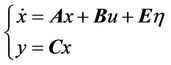
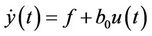
To extend FDI to the processes beyond the scope of existing methods, consider a nonlinear dynamic system that can be described by
 (1)
(1)
where  denotes the nth time derivative of y, f, short for
 is a lumped nonlinear timevarying function of the plant dynamics and the unknown external disturbance d, u is the system’s input and b is a constant. In all physical systems, f and b are both bounded. From fault diagnosis point of view, the f can be thought of lumped unknown un-modeled or incorrectly modeled dynamics combined with the unknown external disturbances. Instead of separating un-modeled dynamics from the disturbance, the term f in its totality is to be estimated as an extended state of the system, together with the states of the system. Normally, an observer only provides the state estimation; but with what is known as Extended State Observer (ESO) [16-19], the term f is treated as another state and estimated in real time. Such additional information proves to be crucial for the FDI purposes, as will be shown in this paper. The ESO technique first developed by Han [16,17], however, is rather complex and its implementation requires the adjustments or tuning of several parameters, which can be difficult and time consuming. Later, Gao [18] improved the ESO technique and made it more practical by using a particular parameterization method that reduces the number of tuning parameters to one. Such parameterized ESO has been successfully applied in many applications, particularly in the context of the Active Disturbance Rejection Control (ADRC) [19].
Based on the parameterized ESO, a new FDI technique is proposed in this paper, which is organized as follows. Section 2 describes the design of the improved ESO and its estimation error convergence. Section 3 presents a case study on a MIMO nonlinear dynamic system. Section 4 describes fault detection by means of the ESO, while Section 5 describes fault isolation, fault identification and degree-of-fault determination. Section 6 gives conclusions about the presented technique.
2. Extended State Observer
In this section, the design of the improved extended state observer (ESO) is described, followed by the proof of the observer’s estimation error convergence.
2.1. Extended State Observer Design
The main idea of ESO is to use an augmented state space model of Equation (1) that includes f as an additional state. Thus, Equation (1) can be represented in state space form as
 (2)
(2)
where both f and η are assumed unknown.
Alternatively, in the case of single output (i.e. y = x1), Equation (2) can be written in matrix form as
 (3)
(3)
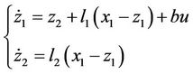
where
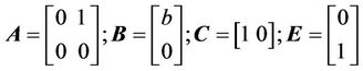
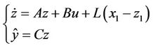
The ESO can be expressed in matrix form as
 (4)
(4)
or
 (5)
(5)
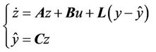
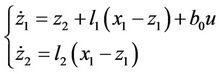
where  is the observer gain vector which can be obtained using any known method such as the pole placement technique. When it is properly selected, the ESO provides an estimate of the state in Equation (3) (i.e. zi estimates xi, where i = 1, 2), where
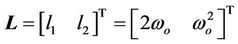
  is the estimate of system output y. More specifically, z1 tracks the system output, while z2 tracks f which includes system internal dynamics and external disturbance. The choice of the observer gain vector L, originally consisted of a set of nonlinear gains [16,17], was simplified with linear gains so that it can be parameterized by solving the characteristic equation of the observer [18]. For instance, if gains are chosen as
 , then the characteristic polynomial of Equation (4) becomes
 (6)
(6)
where ωo is the observer bandwidth, which needs to be tuned in practice to ensure that the ESO operates effecttively, and this is a complex argument (Laplace’s variable). In comparison with the original extended state observer, this is regarded as the improved extended state observer since the observer bandwidth is the only parameter needs to be tuned. The analysis of ESO was briefly given in [18]; a more elaborate account is given in [19]. For practitioners, however, perhaps it is just as interesting to see the various applications of ESO and their success in providing a practical solution in dealing with uncertainties [18,20]. The estimation error of the ESO is described in the next section.
2.2. Estimation Error Convergence
In this section, we will mathematically prove that, with plant dynamics largely unknown, the ESO can accurately estimate the unknown dynamics and disturbances with upper-bounded estimation error. Let
 (7)
(7)
From Equations (2) and (4), the observer estimation error for states x1 ad x2 can be described as
 (8)
(8)
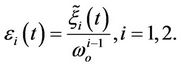
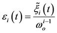
Now let us scale down the observer estimation error  by
by , i.e., let
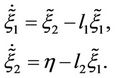
Then, Equation (8) can be written as
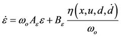 (9)
(9)
where
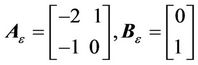
here A is Hurwitz for
 .
.
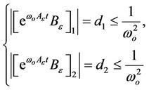
Theorem 1: Assuming  is bounded, then there exists a constant
  and a finite time
  such that
  and
and
Note that
 (10)
(10)
where O is a function representing the order of the reciprocal of bandwidth to the order of a positive integer k. The boundedness of  (i.e.
(i.e. ) means that the rate of change of the combined effect of internal dynamics and external disturbances is finite, which leads to an assumption that the combined effect and the control input are continuous. Here h is essentially the derivative of acceleration. In a typical motion system, h being bounded means that the force applied to the body does not change infinitely within a very short period of time. In other words, the jerk (i.e. time derivative of acceleration) is finite. This is a reasonable assumption for a typical motion.
Proof: Solving (9), gives
 (11)
(11)
Let
 (12)
(12)
Since  is bounded, that is,
 where
where  is a positive constant, for
  then
then
 (13)
(13)
With

the following can be written
 (14)
(14)
Since  is Hurwitz, there exists a finite time
  such that
 (15)
(15)
for all . Hence
 (16)
(16)
for all 
 depends on
  Combining

and Equation (16) which means
gives the following expression
 (17)
(17)
for all  Equation (13) can be expressed in terms of Equations (14) and (17) as follows.
 (18)
(18)
for all  Let
Let
 it follows that
 (19)
(19)
for all  Equation (11) yields the following constraint
 (20)
(20)
Substituting
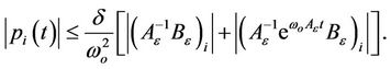
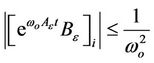
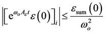
and Equation (18) into (20) leads to a conclusion that the absolute estimation error is, indeed, upper-bounded.
 (21)
(21)
for all 
Theorem 1 has been mathematically proved that, in the absence of the plant model, the estimation error of the ESO as described in Equation (4) is bounded and its upperbound monotonously decreases with the observer bandwidth. As long as the bandwidth is sufficiently large, the ESO can be used to estimate the state as well as the extended state f which includes system internal dynamics and external disturbance. The ESO’s ability to estimate and track the system’s output state, y and the extended state, f provides foundation for the proposed fault detection and isolation schemes. Since the extended state f, which includes system internal dynamics and external disturbances, is estimated by the ESO in real time and cancelled in the control law in real time, the ESO achieves high disturbance rejection performance and strong robustness performance.
3. Case Study: Three-Tank System
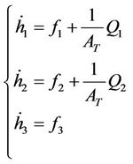
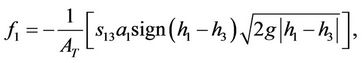
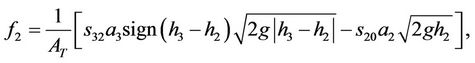
To illustrate how the presented ESO can be used to track a nonlinear dynamic system. A three-tank nonlinear dynamic system [3] as shown in Figure 1 was chosen for a case study. The system consists of three tanks (T1, T2 and T3) that are connected by three pipes. The system has two controlled inputs (pump flow rates), three measurable outputs h1, h2 and h3 (water levels), and three possible faults (pipe blockages). It is, indeed, a strongly coupled multi-inputs multi-outputs (MIMO) system.
Using the Torricelli’s law, the following three dynamic system equations can be obtained
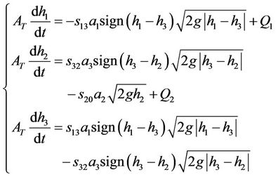 (22)
(22)
where AT is the circular cross-sectional area of each tank (assumed same for all); a1, a2, a3: the circular cross-sec-
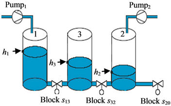
Figure 1. Schematic diagram of the three-tank system.
tion area of each pipe; s13, s32, s20: pipe blockage; Q1, Q2: pump’s flow rate; h1, h2 and h3 denote the water level of tanks T1, T2 and T3, respectively.
The blockage is in terms of degree of fault between 0 and 1, where 0 and 1 correspond to complete blockage and no blockage, respectively. Equation (22) can be rewritten as
 (23)
(23)
where

Let y(t) and u(t) be the system’s output and input vector, respectively,
 (24)
(24)
where h1, h2 and h3 denote the water level of tanks T1, T2 and T3, respectively, and Q1 and Q2 denote the flow rate of pumps 1 and 2, respectively. Essentially, the water levels are the system output variables and the flow rates are the system input variables. Combining Equations (23) and (24), gives
 (25)
(25)
where

The f1, f2 and f3 are called the Generalized System Dynamics of tank T1, T2 and T3, respectively, and u(t) is the system’s inputs. Note that the constant bo can be determined by the system, which in this case, is simply the reciprocal of the tank’s area.
Equation (25) can be represented in state space form as
 (26)
(26)
where

is the system input,
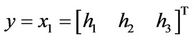
is the system output,

is an augmented state, and ν is the time derivative of f. Rewriting Equation (26) in matrix form, gives
 (27)
(27)
where
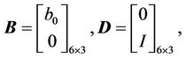

and I is a three-by-three identity matrix. Note that the expression for C in Equation (27) is for three outputs, while that for C in Equation (3) is for single output.
Employing the ESO design (Equations (2)-(6)), denoting y as the measured or actual output,
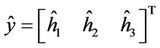
as the estimated output, and incorporating the difference between the two outputs, the ESO of Equation (26) can be rewritten as
 (28)
(28)
The state space observer can be constructed as
 (29)
(29)
where 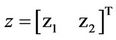 (i.e.
(i.e.  and
and  ).
).
Equation (22) shows that three-tank system consists of three simultaneous first-order differential equations. Thus, the observer gain matrix, L can be expressed as
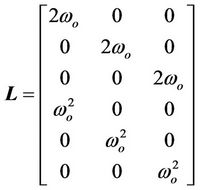 (30)
(30)
With a chosen bandwidth ωo, the z vector can be used to estimate the system outputs and the system dynamics in real time. As proved in Sec. 2.2, the ESO’s estimation error is upper-bounded and monotonously decreases with the bandwidth. With a sufficiently large bandwidth and as time proceeds, z1 quickly approaches y (i.e. h1, h2 and h3), and z2 approaches f (i.e. f1, f2 and f3). In other words, z1 tracks the system’s outputs, and z2 tracks the un-modeled system dynamics combined with external disturbance. More specifically, as stated in Equation (29) estimates the state variables x1 (i.e. the water level h1, h2 and h3), and
  estimates the extended state f (i.e. f1, f2 and f3).
 (31)
(31)
The value of the bandwidth ωo affects the system’s tracking speed and the state estimation’s sensitivity to measurement noise. Figures 2 and 3 show the simulation results on the sensitivity of the ωo value to the measurement noise (with sampling time, Δt = 0.01 sec).
The simulation results demonstrate the effectiveness of the ESO in tracking the outputs and the dynamics of the system. The smaller the ωo is, the slower the ESO tracks the system. As the ωo increases, the ESO tracks the system more quickly, but it also becomes more sensitive to

Figure 2. System dynamics tracking with ωo = 1 and 5% noise.
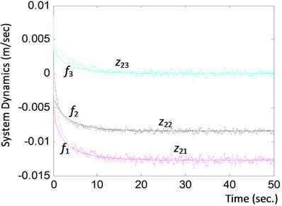
Figure 3. System dynamics tracking with ωo = 5 and 5% noise.
the measurement noise. Choosing the appropriate ωo is a trade-off between the tracking speed and sensitivity to noise.
4. Fault Detection by Means of ESO
This section presents how faults can be detected by means of the Extended State Observers based on realtime estimation of the system dynamics.
4.1. Basic Fault Detection Scheme
As mentioned earlier, the faults to be detected are neither the sensor faults nor the actuator faults. Rather, they are the process faults possibly caused by structural deterioration. The process faults, in this case, are the pipe blockage faults, s13, s32 and s20 as shown in Figure 1. Traditionally, faults are considered detected when the outputs exceed the expected values by a preset tolerance. This approach, however, has some drawbacks in open-loop and closed-loop controls. When using the ESO for closed-loop control, observing the system’s output does not provide useful information about the health of the system because the controller tries to augment the inputs in an effort to stabilize the system. Thus, the health does not surface until the system finally collapses. Using the ESO for open-loop control also encounters a problem before the system reaches its steady states. In other words, an abrupt change on the system output does not necessarily mean the system is becoming faulty. Thus, solely relying on monitoring the system output could trigger a false alarm or miss detection of possible faults.
It is worthwhile to note that the ESO’s unique feature is its ability to estimate the general system dynamics (i.e. the un-modeled system dynamics and unknown external disturbance) in real time, which provides crucial information for the presented fault detection technique. Our study found that the system outputs and the general system dynamics both exhibit abrupt changes as soon as a fault occurs. However, the rate of change on the general system dynamics is more profound. Furthermore, the system outputs potentially contain the process faults (such as the pipe blockage faults) as well as the actuator faults (such as the actuating faults in the pumps), while the general system dynamics contains solely the process faults. Since the goal of this study was to diagnose the process faults, our proposed fault detection scheme is based on the general system dynamics, f. More specifically, a fault is considered detected when the rate of change of general system dynamics,  exceeds the predetermined threshold value.
4.2. Fault Detection without Exact Knowledge of the Plant Model
As mentioned earlier, the ESO estimates the states of z21, z22 and z23 which track the system dynamics f1, f2 and f3. The only information need for fault detection is to estimate the value of bo. Our study found that the value of bo is, indeed, not critical to fault detection. Figure 4 shows the simulation result of successfully detecting two sequential faults using the exact bo values of 127. Figure 5 further indicates the same faults can be detected even with bo value of 635, which is five times as much as the exact one. The simulation assumes that the first blockage fault s13 = 0.8 (i.e. 80% blocked) in the pipe connecting tanks 1 and 3 occurs at t = 10 sec., followed by the second blockage fault s32 = 0.6 (i.e. 60% blocked) in the pipe connecting tanks 3 and 2 occurring at t = 20 sec. The first fault affects the dynamics of tanks 1 and 3 (f1 and f3), which reflects the abrupt changes in the estimated states z21 and z23. The second fault affects the dynamics of tanks 3 and 2 (f3 and f2), which reflects abrupt changes in the estimated states z23 and z22.
Note that ESO’s estimated z21, z22 and z23 closely track the system dynamics, f1, f2 and f3, respectively. The bo
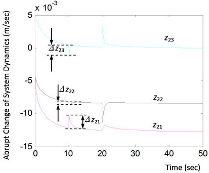
Figure 4. Detection of multiple faults (s13 = 0.8 at t = 10 sec and s32 = 0.6 at t = 20 sec) with bo = 127 (the exact value).
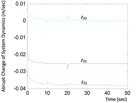
Figure 5. Detection of multiple faults (s13 = 0.8 at t = 10 sec and s32 = 0.6 at t = 20 sec) with bo = 635 (Rough estimated value).
value is associated with the physical system, which is the cross-sectional area of the pipes connecting tanks. Figures 4 and 5 clearly demonstrate that the bo value is not critical to fault detection, which suggests that knowledge of the exact system model is not required.
The presented ESO-based fault detection technique suggests that the accuracy of bo is not critical to fault detection. It should be noted that although faults can be detected without exact knowledge of the plant model, some knowledge about the model, such as the order of the system, is needed.
The changes of these three extended states are worth of observing. For instance, as shown in Figure 4, when the first fault just occurred, ∆z23 was negative, ∆z22 was close to 0, and ∆z21 was positive. But, when the second fault was added 10 seconds later, the ∆z23 became positive and the ∆z22 became negative, but the ∆z21 remained positive but smaller. The changing signs of the states and the levels of the state values (i.e. low, medium and high) provide useful information for fault isolation.
5. Fault Isolation and Fault Identification
The fault isolation to be presented here is based on the assumption that the exact system model is unknown. However, in order to verify the effectiveness of the presented technique, the referenced system outputs need to be generated first.
5.1. Generation of Reference Values
The outputs, in the case of the three-tank system, can be obtained by using such as piezo-resistive pressure sensors with resolution of 0.1 mm to measure the water levels. With sufficient input-output correspondence, a backpropagation neural network can be trained. The trained network can then be used to predict the outputs with reasonably good accuracy.
Alternatively, the system outputs can be estimated in real-time using the ESO based on the assumption that the exact plant model is known. With this alternative approach, the first step for identifying faults is to associate all faults with the system dynamics. First of all, Equation (22) containing the pipe dynamics (the dynamics between two outputs) can be extracted as follows.
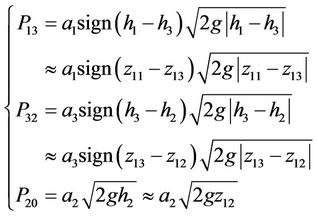 (32)
(32)
where z11, z12 and z13 are the ESO’s system outputs, the water level in each tank as shown in Equation (29). Substituting Equations (32) into (23), gives the expressions for the general system dynamics f as follows:
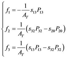 (33)
(33)
where AT is the circular cross-sectional area of each tank (assumed same for all). Note that bo is reciprocal of the AT.
Furthermore, if the exact plant model were known, the degree of each fault for the three-tank system could be easily determined by
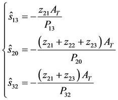 (34)
(34)
In the case of uncertain plant model, not only fault isolation becomes more difficult, degree-of-fault determination also becomes a major task. These will be addressed in the following two sections.
5.2. Fault Isolation by Means of Fuzzy Inference and ESO
In addition to monitoring the system outputs, the system dynamics, f, used for fault detection can be used for fault isolation. Referring to Figure 4 when the first fault occurs at t = 10 sec., if Δz21 (the ESO’s estimated ∆f1) is positive, Δz22 (the ESO’s estimated ∆f2) is negative, and Δz23 (the ESO’s estimated ∆f3) is negative, then a blockage fault between tanks 1 and 3 (i.e. s13) likely has occurred. When the second fault occurs at t = 20 sec., if Δz21 is positive, Δz22 is negative and Δz23 is positive, then a blockage fault between tanks 3 and 2 (i.e. s32) likely has occurred. The observations suggest some intuitive logic, better known as fuzzy logic can be employed to classify the faults.
A fuzzy inference system (FIS) consists of input membership functions, output membership functions and the if-then fuzzy logic rules. Among them, constructing the proper input membership functions is critical, and can be most difficult if there is no prior knowledge about how input data are distributed. The best way to determine data distribution is through the use of histograms. The FSI’s inputs variables are Δz21, Δz22 and Δz23 which are normalized to the range of [–1,1]. The output variables are the degree of fault for s13, s32, s20, which are normalized to the range of [0,1], where “0” represents no fault, and “1” represents complete fault.
The input membership functions for Δz21, Δz22 and Δz23 are the same, which are LNG (Large Negative), SNG (Small Negative) and POS (Positive). The output membership functions for faults s13, s32 and s20 are also the same, which are Normal and Faulty. The crisp input variables are first fuzzified and then processed by the fuzzy logic rules. Afterward, they are defuzzified into the range between 0 and 1, which indicates the fault occurrence confidence between 0% and 100%. The six if-then fuzzy rules for a single fault are
Rule 1: If (Δz21 is POS) and (Δz22 is SNG) and (Δz23 is LNG) then (s13 is Faulty) and (s32 is Normal) and (s20 is Normal)
Rule 2: If (Δz21 is POS) and (Δz22 is LNG) and (Δz23 is LNG) then (s13 is Faulty) and (s32 is Normal) and (s20 is Normal)
Rule 3: If (Δz21 is POS) and (Δz22 is LNG) and (Δz23 is SNG) then (s13 is Faulty) and (s32 is Normal) and (s20 is Normal)
Rule 4: If (Δz21 is POS) and (Δz22 is LNG) and (Δz23 is POS) then (s32 is Faulty) and (s13 is Normal) and (s20 is Normal)
Rule 5: If (Δz21 is POS) and (Δz22 is SNG) and (Δz23 is POS) then (s32 is Faulty) and (s13 is Normal) and (s20 is Normal)
Rule 6: If (Δz21 is POS) and (Δz22 is POS) and (Δz23 is POS) then (s20 is Faulty) and (s13 is Normal) and (s32 is Normal)
POS: Positive; SNG: Small negative; LNG: Large negative.
The FIS essentially gives the confidence in a fault occurrence. A component is considered faulty when the confidence exceeds or equal to 80%.
5.3. Fault Identification via Neural Networks
With the given three-tank system, incipient faults are likely to occur, which will require monitoring and determining the degree of fault at all time. However, degree of fault, in theory, cannot be determined unless the exact plant model is known. The only alternative is to use experimental data. In absence of experimental data, simulation data using Equation (2) were generated.
Table 1 shows examples of single fault in which the fuzzy inference system was able to isolate all the faults with 96% confidence which was the maximum output value by design. The error of each predicted degree of fault was extremely small. In this simulation, the system input variables are the pump rates: Q1 = 6 liters/min and Q2 = 4 liters/min. To demonstrate the ESO’s effectiveness in filtering noise, 5% white noise was added to each

Table 1. Result of fault identification and isolation.
input variable.
With the given three-tank system, incipient faults are likely to occur, which will require monitoring and determining the degree of fault at all time. However, degree of fault, in theory, cannot be determined unless the exact plant model is known. The only alternative is to use experimental data. In absence of experimental data, simulation data using Equation (2) were generated.
To do so, a back-propagation neural network for each fault using randomly selected inputs and their corresponding outputs was trained via Matlab Neural Network Toolbox. The input variables of each neural network are the pump flow rates, while the output variable is the degree of fault between 0 and 1. As soon as the fault is isolated, the respective neural network (NN) is fired to instantly predict the degree of fault.
Table 1 shows examples of single fault in which the fuzzy inference system was able to isolate all the faults with 96% confidence which was the maximum output value by design. In this simulation, the system input variables: the pump rates Q1 and Q2 are liters/min. To demonstrate the ESO’s effectiveness in filtering noise, 5% white noise was added to each input variable. More studies on model-free fault diagnosis can be found in [21-23].
6. Conclusions and Future Work
This study mathematically proves that the ESO’s estimation error is upper-bounded and its upper-bound monotonously decreases with the observer bandwidth. This important proof allows for applying the improved Extended State Observer (ESO) to be an effective means for fault detection and isolation (FDI). The main advantage of the presented FDI technique is its robustness against uncertainty in the plant dynamics as well as disturbances. The parameterized ESO that requires tuning of only a single parameter (the observer bandwidth) makes it easy to be implemented in fault diagnosis. The bandwidth affecting the system’s tracking speed and sensitivity to measurement noise can be easily tuned to meet the individual need for diagnosis.
From the model-based FDI point of view, the issue of how much knowledge about a nonlinear dynamic system is needed has been of great interest to researchers for years. This study concludes that the ESO-based fault detection requires little knowledge about the plant model, not much beyond the order of the system.
The ESO-based fuzzy inference proved to be an effecttive mean for fault isolation. The fuzzy inference is particularly good at handling uncertainty in the plant model. Furthermore, this study went beyond the traditional FDI by adding the capability of determining the degree of fault via neural networks. Such capability is particularly important for diagnosis of incipient faults.
The contributions of the presented process fault diagnosis technique are summarized as follows:
1) The improved ESO made it easy to tune only a single parameter, the observer’s bandwidth. The selection of an appropriate bandwidth could effectively filter the measurement noise and control the desired tracking speed.
2) In addition to tracking and estimating the system outputs, the extended/augmented state of the ESO could be used to track and estimate the un-modeled or incurrectly modeled system dynamics in real time, which provides useful information for the fault detection.
3) The ESO’s estimation error was mathematically proved to be upper-bounded. This proof was critical for enabling the ESO to accurately track and estimate the system dynamics.
4) Combining the ESO with fuzzy inference for fault isolation is a new attempt, which is particularly useful when the exact plant model is unknown.
5) Unlike sensor faults or actuator faults, process faults such as the blockage faults in the three-tank system affect only the system dynamics, f, which can be detected when an abrupt change in the system dynamics is observed.
The simulation result shows the identified faults are in full agreement with the assumed faults. In the future, we plan to conduct an experimental study to verify the presented technique.
REFERENCES
- P. M. Frank, S. X. Ding and T. Marcu, “Model-Based Fault Diagnosis in Technical Processes,” Transaction of Institute of Measurement and Control, Vol. 22, No. 1, 2000, pp. 57-101.
- V. Venkatasubramanian, R. Rengaswamy, K. Yin and S. N. Kavuri, “A Review of Process Fault Detection and Diagnosis: Part I. Quantitative Model-Based Methods,” Computer and Chemical Engineering, Vol. 27, No. 3, 2003, pp. 293-311. doi:10.1016/S0098-1354(02)00160-6
- P. P. Lin and X. Li, “Fault Diagnosis, Prognosis and SelfReconfiguration for Nonlinear Dynamic System Using Soft Computing Techniques,” Proceedings of IEEE Conference on Systems, Man and Cybernetics, Taipei, 14-16 December 2006.
- R. Tarantino, F. Szigeti and E. Colina-Morles, “Generalized Luenberger Observer-Based Fault-Detection Filter Design: An Industrial Application,” Control Engineering Practice, Vol. 8, 2000, pp. 665-671. doi:10.1016/S0967-0661(99)00181-1
- S. K. Dash, R. Rengaswamy and V. Venkatasubramanian, “Fault Diagnosis in a Nonlinear CSTR Using Observers,” Annual AIChE Meeting, Reno, 2001, p. 282i.
- A. Z. Sotomayor and D. Odloak, “Observer-Based Fault Diagnosis in Chemical Plants,” Chemical Engineering Journal, Vol. 112, 2005, pp. 93-108. doi:10.1016/j.cej.2005.07.001
- P. M. Frank, “Advanced Fault Detection and Isolation Schemes Using Nonlinear and Robust Observers,” 10th IFAC World Congress, Munich, 27-31 July 1987.
- P. M. Frank, “Online Fault-Detection in Uncertain Nonlinear-Systems Using Diagnostic Observers: A Survey,” International Journal of Systems Science, Vol. 25, No. 12, 1994, pp. 2129-2135. doi:10.1080/00207729408949341
- P. M. Frank and X. Ding, “Survey of Robust Residual Generation and Evaluation Methods in Observer-Based Fault Detection Systems,” Journal of Process Control, Vol. 7, No. 6, 1997, pp. 403-424. doi:10.1016/S0959-1524(97)00016-4
- R. Isermann, “Model-Based Fault-Detection and Diagnosis—Status and Applications,” Annual Reviews in Control, Vol. 29 2005, pp. 71-85. doi:10.1016/j.arcontrol.2004.12.002
- V. F. Filareretov, M. K. Vukobratovic and A. N. Zhirabok, “Observer-Based Fault Diagnosis in Manipulation Robots,” Mechatronics, Vol. 9, 1999, pp. 929-939. doi:10.1016/S0957-4158(99)00017-3
- A. Xu and Q. Zhang, “Nonlinear System Fault Diagnosis Based on Adaptive Estimation,” Automatica, Vol. 40, 2004, pp. 1181-1193. doi:10.1016/j.automatica.2004.02.018
- M. Fang, Y. Tian and L. Guo, “Fault Diagnosis of Nonlinear System Based on Generalized Observer,” Applied Mathematics and Computation, Vol. 185, 2007, pp. 1131- 1137. doi:10.1016/j.amc.2006.07.034
- H. B. Wang, J. L. Wang and J. Lam, “Robust Fault Detection Observer Design: Iterative LMI Approaches,” ASME Journal of Dynamic Systems, Measurement, and Control, Vol. 129, 2007, pp. 77-82. doi:10.1115/1.2397155
- A. Radke, “On Disturbance Estimation and Its Application on Health Monitoring,” Doctoral Dissertation, Cleveland State University, 2006.
- J. Han, “A Class of Extended State Observers for Uncertain Systems,” Control and Decision, Vol. 10, No. 1, 1995, pp. 85-88.
- J. Han, “Nonlinear Design Methods for Control Systems,” Proceeding of the 14th IFAC World Congress, Beijing, 4-9 July 1999.
- Z. Gao, “Scaling and Parameterization Based Controller Tuning,” Proceedings of American Control Conference, Denver, 4-6 June 2003, pp. 4989-4996.
- Q. Zheng, L.Q. Gao and Z. Gao, “On Estimation of Plant Dynamics and Disturbance from Input-Output Data in Real Time,” Proceedings of the IEEE Multi-Conference on Systems and Control, Singapore City, 1-3 October 2007, pp. 1167-1172.
- Z. Gao, “Active Disturbance Rejection Control: A Paradigm Shift in Feedback Control System Design,” Proceedings of American Control Conference, Minneapolis, 14-16 June 2006, pp. 4989-4996.
- P. P. Lin and H. Singh, “Intelligent Model-Free Diagnosis for Multiple Faults in a Nonlinear Dynamic System,” Proceedings of IEEE/ASME Conference on Advanced Intelligent Mechatronics (AIM), Zurich, 4-7 September 2007.
- P. Zhang and S. Ding, “A Model-Free Approach to Fault Diagnosis of Continuous-Time Systems Based on Time Domain Data,” International Journal of Automation and Computing, Vol. 4, No. 2, 2007, pp. 189-194. doi:10.1007/s11633-007-0189-y
- M. Kowal and J. Korbicz, “Fault Detection under Fuzzy Model Uncertainty,” International Journal of Automation and Computing, Vol. 4, No. 2, 2007, pp. 117-124. doi:10.1007/s11633-007-0117-1