Journal of Modern Physics
Vol.4 No.6A(2013), Article ID:33596,32 pages DOI:10.4236/jmp.2013.46A008
Correlated-Electron Systems and High-Temperature Superconductivity
1Electronics and Photonics Research Group, National Institute of Advanced Industrial Science and Technology (AIST), Tsukuba Central 2, Tsukuba, Japan
2Hakodate National College of Technology, Hakodate, Japan
Email: t-yanagisawa@aist.go.jp
Copyright © 2013 Takashi Yanagisawa et al. This is an open access article distributed under the Creative Commons Attribution License, which permits unrestricted use, distribution, and reproduction in any medium, provided the original work is properly cited.
Received April 2, 2013; revised May 5, 2013; accepted June 1, 2013
Keywords: High-Temperature Superconductivity; Strongly Correlated Electrons; Monte Carlo Methods; Hubbard Model; Condensation Energy; Pair-Correlation Function
ABSTRACT
We present recent theoretical results on superconductivity in correlated-electron systems, especially in the twodimensional Hubbard model and the three-band d-p model. The mechanism of superconductivity in high-temperature superconductors has been extensively studied on the basis of various electronic models and also electron-phonon models. In this study, we investigate the properties of superconductivity in correlated-electron systems by using numerical methods such as the variational Monte Carlo method and the quantum Monte Carlo method. The Hubbard model is one of basic models for strongly correlated electron systems, and is regarded as the model of cuprate high temperature superconductors. The d-p model is more realistic model for cuprates. The superconducting condensation energy obtained by adopting the Gutzwiller ansatz is in reasonable agreement with the condensation energy estimated for YBa2Cu3O7. We show the phase diagram of the ground state using this method. We have further investigated the stability of striped and checkerboard states in the under-doped region. Holes doped in a half-filled square lattice lead to an incommensurate spin and charge density wave. The relationship of the hole density  and incommensurability
 ,
,  , is satisfied in the lower doping region, as indicated by the variational Monte Carlo calculations for the two-dimensional Hubbard model. A checkerboard-like charge-density modulation with a roughly
  period has also been observed by scanning tunneling microscopy experiments in Bi2212 and Na-CCOC compounds. We have performed a variational Monte Carlo simulation on a two-dimensional
  -
- -
- -
- Hubbard model with a Bi-2212 type band structure and found that the
  period checkerboard spin modulation, that is characterized by multi Q vectors, is indeed stabilized. We have further performed an investigation by using a quantum Monte Carlo method, which is a numerical method that can be used to simulate the behavior of correlated electron systems. We present a new algorithm of the quantum Monte Carlo diagonalization that is a method for the evaluation of expectation value without the negative sign problem. We compute pair correlation functions and show that pair correlation is indeed enhanced with hole doping.
1. Introduction
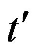
The effect of the strong correlation between electrons is important for many quantum critical phenomena, such as unconventional superconductivity (SC) and the metalinsulator transition. Typical correlated electron systems are high-temperature superconductors [1-5], heavy fermions [6-9] and organic conductors [10]. The phase diagram for the typical high-Tc cuprates is shown in Figure 1 [9]. It has a characteristics that the region of antiferromagnetic order exists at low carrier concentrations and the superconducting phase is adjacent to the antiferromagnetism.
In the low-carrier region shown in Figure 2, there is the anomalous metallic region where the susceptibility and  show a peak above Tc suggesting an existence of the pseudogap. To clarify an origin of the anomalous metallic behaviors is also a subject attracting many physicists as a challenging problem.
It has been established that the Cooper pairs of high-Tc cuprates have the  -wave symmetry in the hole-doped materials [11,12]. Several evidences of
  -wave pairing
Figure 1. Phase diagram delineating the regions of superconductivity and antiferromagnetic ordering of the Cu2+ ions for the hole-doped La2–xSrxCuO4 and electron-doped Nd2–xCexCuO4–y systems.

Figure 2. Phase diagram showing the regions of non-Fermi liquid and pseudogap metal for the hole-doped case. The boundaries indicated in the figure are not confirmed yet.
symmetry were provided for the electron-doped cuprates Nd2–xCexCuO4 [13-15]. Thus it is expected that the superconductivity of electronic origin is a candidate for the high-Tc superconductivity. We can also expect that the origin of  -wave superconductivity lies in the onsite Coulomb interaction of the two-dimensional Hubbard model.
The antiferromagnetism should also be examined in correlated electron systems. The undoped oxide compounds exhibit rich structures of antiferromagnetic correlations over a wide range of temperature that are described by the two-dimensional quantum antiferromagnetism [16-18]. A small number of holes introduced by doping are responsible for the disappearance of long-range antiferromagnetic order [19-24].
Recent neutron scattering experiments have suggested an existence of incommensurate ground states with modulation vectors given by 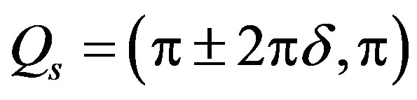 and
and 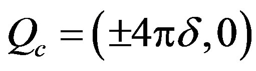 (or
(or 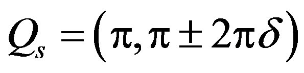 and
and 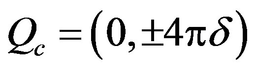 ) where
  denotes the hole-doping ratio [25]. We can expect that the incommensurate correlations are induced by holes doped into the Cu-O plane in the underdoped region. A checkerboard-like charge-density modulation with a roughly
  period has also been observed by scanning tunneling microscopy experiments in Bi2212 and Na-CCOC compounds.
Recently the mechanism of superconductivity in hightemperature superconductors has been extensively studied using various two-dimensional (2D) models of electronic interactions. Among them the 2D Hubbard model [26] is the simplest and most fundamental model. This model has been studied intensively using numerical tools, such as the Quantum Monte Carlo method [27-42], and the variational Monte Carlo method [24,43-50]. The two-leg ladder Hubbard model was also investigated with respect to the mechanism of high-temperature superconductivity [51-59].
Since the discovery of cuprate high-temperature superconductors, many researchers have tried to explain the occurrence of superconductivity of these materials in terms of the two-dimensional (2D) Hubbard model. However, it remains matter of considerable controversial as to whether the 2D Hubbard model accounts for the properties of high-temperature cuprate superconductors. This is because the membership of the the two-dimensional Hubbard model in the category of strongly correlated systems is a considerable barrier to progress on this problem. The quest for the existence of a superconducting transition in the 2D Hubbard model is a long-standing problem in correlated-electron physics, and has been the subject of intensive study [35,36,38,46, 60,61]. In particular, the results of quantum Monte Carlo methods, which are believed to be exact unbiased methods, have failed to show the existence of superconductivity in this model [38,61].
In the weak coupling limit we can answer this question. We can obtain the superconducting order parameter of the Hubbard model in the limit of small , that is given by [62-66]
 (1)
(1)
where  is the strength of the on-site Coulomb interaction and the exponent
  is determined by solving the gap equation. Thus the existence of the superconducting gap is guaranteed by the weak coupling theory although
  is extremely small because of the exponential behavior given above.
  indicates the strength of superconductivity. In the intermediate or large coupling region, we must study it beyond the perturbation theory.
We investigate the ground state of the Hubbard model by employing the variational Monte Carlo method. In the region , the finite superconducting gap is obtained by using the quantum variational Monte Carlo method. The superconducting condensation energy obtained by adopting the Gutzwiller ansatz is in reasonable agreement with the condensation energy derived for YBa2Cu3O7. We have further investigated the stability of striped and checkerboard states in the under-doped region. Holes doped in a half-filled square lattice lead to an incommensurate spin and charge density wave. The relationship of the hole density x and incommensurability
 ,
,  , is satisfied in the lower doping region. This is consistent with the results by neutron scattering measurements. To examine the stability of a
  checkerboard state, we have performed a variational Monte Carlo simulation on a two-dimensional
  Hubbard model with a Bi-2212 type band structure. We found that the
  period checkerboard checkerboard spin modulation that is characterized by multi
  vectors is stabilized.
Further investigation has been performed by using the quantum Monte Carlo method which is a numerical method that can be used to simulate the behavior of correlated electron systems. This method is believed to be an exact unbiased method. We compute pair correlation functions to examine a possibility of superconductivity.
The Quantum Monte Carlo (QMC) method is a numerical method employed to simulate the behavior of correlated electron systems. It is well known, however, that there are significant issues associated with the application to the QMC. First, the standard Metropolis (or heat bath) algorithm is associated with the negative sign problem. Second, the convergence of the trial wave function is sometimes not monotonic, and further, is sometimes slow. In past studies, workers have investigated the possibility of eliminating the negative sign problem [37,38,40-42]. We present the results obtained by a method, quantum Monte Carlo diagonalization, without the negative sign problem.
2. Hubbard Hamiltonian
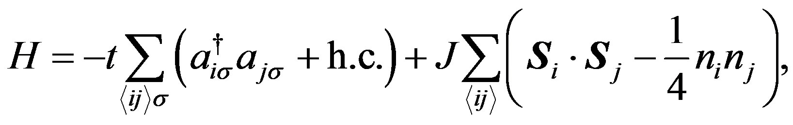
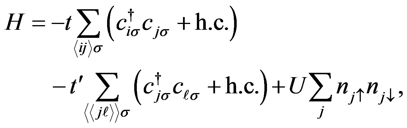
The Hubbard Hamiltonian is
 (2)
(2)
where  and
and  denote the creation and annihilation operators of electrons, respectively, and
  is the number operator. The second term represents the on-site Coulomb interaction which acts when the two electrons occupy the same site. The numbers of lattice sites and electrons are denoted as
  and
and , respectively. The electron density is
 .
.
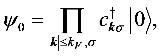
In the non-interacting limit , the Hamiltonian is easily diagonalized in terms of the Fourier transformation. In the ground state each energy level is occupied by electrons up to the Fermi energy. In the other limit
 , each site is occupied by the upor down-spin electron, or is empty. The non-zero
  induces the movement of electrons that leads to a metallic state id
 . The ground state is probably insulating at half-filling
  if
if  is sufficiently large.
If  are non-zero only for the nearest-neighbor pairs, the Hubbard Hamiltonian is transformed to the following effective Hamiltonian for large
  [67]:
[67]:
 (3)
(3)
where  and
and  and
and  indicate the nearest-neighbor sites in the
  and
and  directions, respectively. The second term contains the three-site terms when
 . If we neglect the three-site terms, this effective Hamiltonian is reduced to the t-J model:
where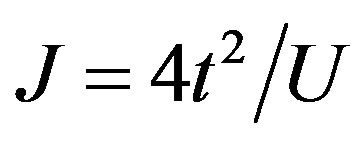 .
.
The Hubbard model has a long history in describing the magnetism of materials since the early works by Hubbard [26], Gutzwiller [68] and Kanamori [69]. Onedimensional Hubbard model has been well understood by means of the Bethe ansatz [70-72] and conformal field theory [73-75]. The solutions established a novel concept of the Tomonaga-Luttinger liquid [76] which is described by the scalar bosons corresponding to charge and spin sectors, respectively. The correlated electrons in twoand three-dimensional space are still far from a complete understanding in spite of the success for the one-dimensional Hubbard model. A possibility of superconductivity is a hot topic as well as the magnetism and metal-insulator transition for the twoand three-dimensional Hubbard model.
The three-band Hubbard model that contains  and
and  orbitals has also been investigated intensively with respect to high temperature superconductors [24,64, 77-88]. This model is also called the d-p model. The 2D three-band Hubbard model is the more realistic and relevant model for two-dimensional CuO2 planes which are contained usually in the crystal structures of high-
 superconductors. The network of CuO2 layer is shown in Figure 3. The parameters of the three-band Hubbard model are given by the Coulomb repulsion
 , energy levels of
  electrons
  and
and  electron
 , and transfer between
  orbitals given by
 . Typical parameter values for the three-band (
 -
- ) Hubbard model are shown in Table 1. The Hamiltonian of the
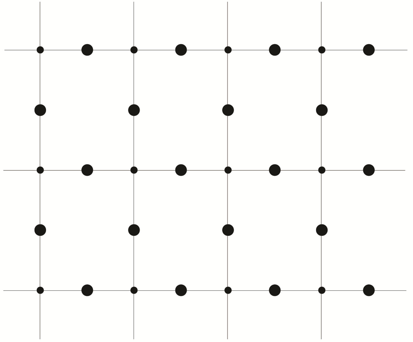
Figure 3. The lattice of the three-band Hubbard model on the CuO2 plane. Small circles denote Cu sites and large ones denote O sites.
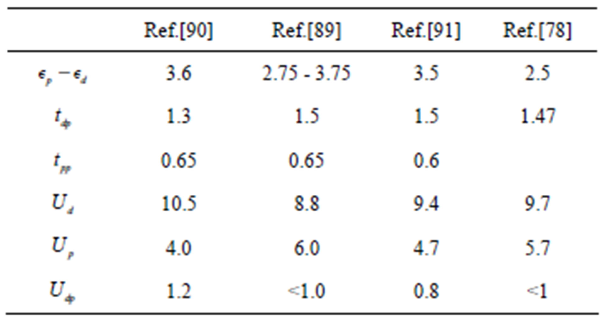
Table 1. Typical parameter values for the three-band Hubbard model. Energies are measured in eV.
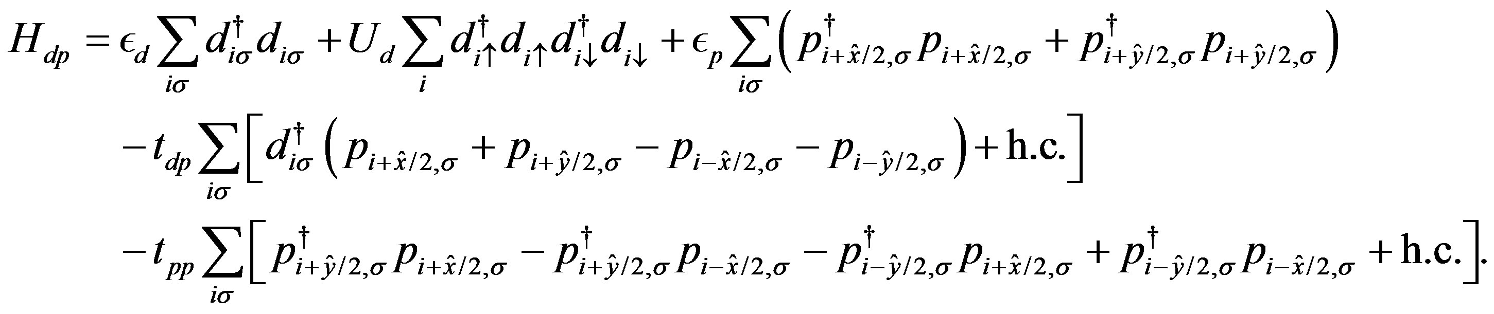
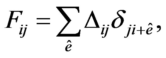
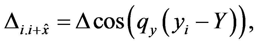
three-band Hubbard model is written as [24,47,48,80] (see Equation (4)) where  and
and  represent unit vectors along x and y directions, respectively.
  and
and  denote the operators for the
  electrons at site
 . Similarly
  and
and  are defined.
  denotes the strength of Coulomb interaction between
  electrons. For simplicity we neglect the Coulomb interaction among
  electrons in this paper. Other notations are standard and energies are measured in
  units. The number of cells is denoted as
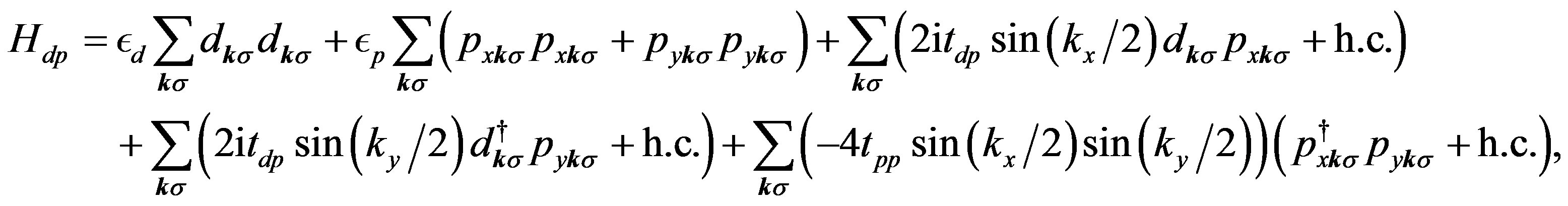
  for the three-band Hubbard model. In the non-interacting case
  the Hamiltonian in the k-space is written as (see Equation (5)).
where 
 ,
, 
 and
and 
are operators for  -,
-,  - and
- and  -electron of the momentum
  and spin
 , respectively.
In the limit ,
,  , and
, and , the
, the  -
- model is mapped to the t-J model with
 (6)
(6)
where .
. 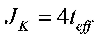 gives the antiferromagnetic coupling between the neighboring
  and
and  electrons. In real materials
  is not so large. Thus it seems that the mapping to the t-J model is not necessarily justified.
3. Variational Monte Carlo Studies
In this Section we present studies on the two-dimensional Hubbard model by using the variational Monte Carlo method.
3.1. Variational Monte Carlo Method
Let us start by describing the method based on the 2D Hubbard model. The Hamiltonian is given by
 (7)
(7)
where  denotes summation over all the nearestneighbor bonds and
  means summation over the next nearest-neighbor pairs.
  is our energy unit. The dispersion is given by
 (8)
(8)
Our trial wave function is the Gutzwiller-projected wave functions defined as
 (9)
(9)
 (10)
(10)
| |
where
 (11)
(11)
 (12)
(12)
 is the Gutzwiller projection operator given by
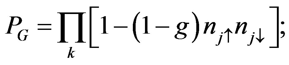 (13)
(13)
 is a variational parameter in the range from 0 to unity and
  labels a site in the real space.
  is a projection operator which extracts only the sites with a fixed total electron number
 . Coefficients
  and
and  in
in  appear in the ratio defined by
 (14)
(14)
where  and
and  is a k-dependent gap function.
  is a variational parameter working like the chemical potential.
  is the Fourier transform of
 . The wave functions
  and
and  are expressed by the Slater determinants for which the expectations values are evaluated using a Monte Carlo procedure [43,44,92].
  is written as
 (15)
(15)
where
 (16)
(16)
Then  is written using the Slater determinants as
 (17)
(17)
where  is the Slater determinant defined by
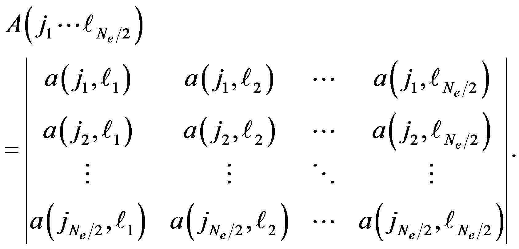 (18)
(18)
In the process of Monte Carlo procedure the values of cofactors of the matrix in Equation (18) are stored and corrected at each time when the electron distribution is modified. We optimized the ground state energy
 (19)
(19)
with respect to ,
,  and
and  for
for  for
for . For
. For  the variational parameter is only
 . We can employ the correlated measurements method [93] in the process of searching optimal parameter values minimizing
 .
.
A Monte Carlo algorithm developed in the auxiliary field quantum Monte Carlo calculations can also be employed in evaluating the expectation values for the wave functions shown above [94-96]. Note that the Gutzwiller projection operator is written as
 (20)
(20)
where . Then using the discrete HubbardStratonovich transformation, the Gutzwiller operator is the bilinear form:
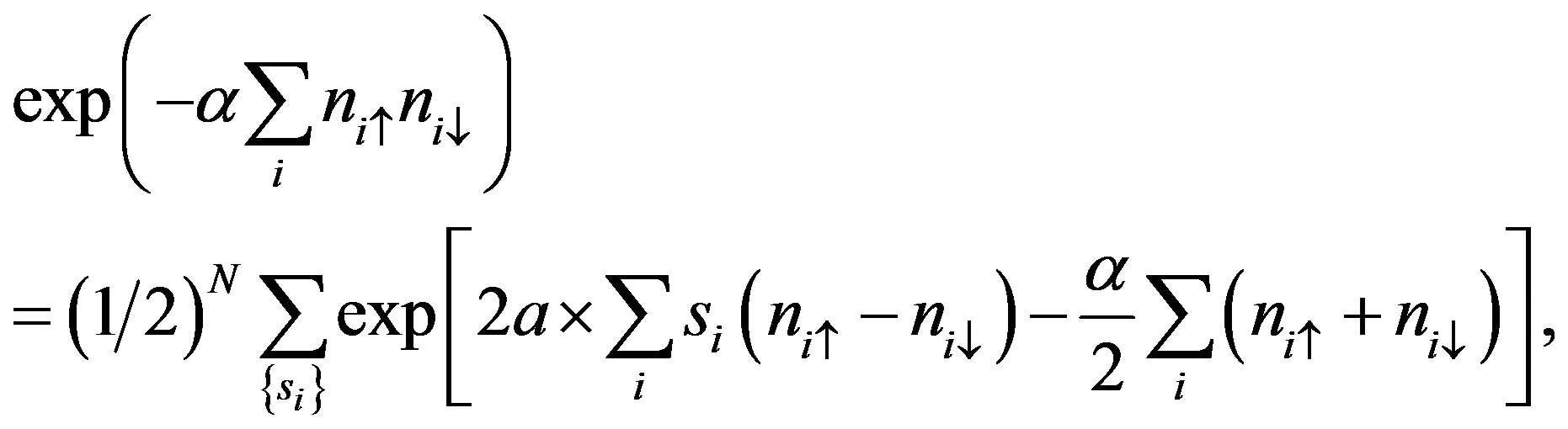 (21)
(21)
where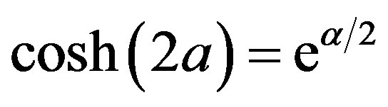 . The Hubbard-Stratonovich auxiliary field
  takes the values of
 . The norm
  is written as
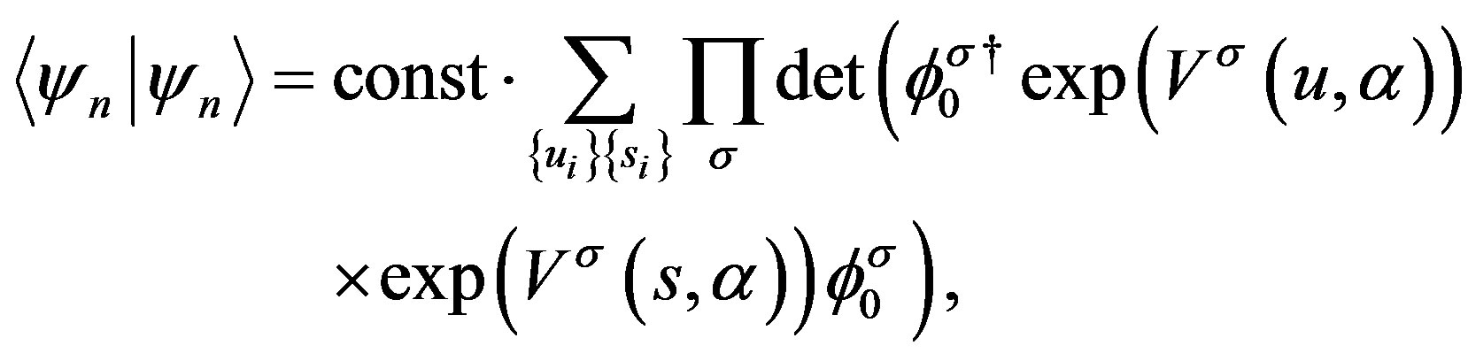 (22)
(22)
where  is a diagonal
  matrix corresponding to the potential
 (23)
(23)
 is written as
 (24)
(24)
where  denotes a diagonal matrix with elements given by the arguments
 . The elements of
 are given by linear combinations of plane waves. For example,
 (25)
(25)
Then we can apply the standard Monte Carlo sampling method to evaluate the expectation values [94,95]. This method is used to consider an off-diagonal Jastrow correlation factor of exp(–S)-type. The results for the improved wave functions are discussed in Section 3.10.
3.2. Superconducting Condensation Energy
We study the cases of the  -, extended
  - (
- ( -) and
  -wave gap functions in the following:
 (26)
(26)
 (27)
(27)
 (28)
(28)
In Figure 4 calculated energies per site with  on the
  lattice are shown for the case of
  and
and  [46].
[46].  is plotted as a function of
  for three types of gap functions shown above. We impose the periodic and the antiperiodic boundary conditions for
  - and
- and  -direction, respectively. This set of boundary conditions is chosen so that
  does not vanish for any k-points occupied by electrons.
  was obtained as the average of the results of several Monte Carlo calculations each with
  steps.
  has minimum at a finite value of
  in the case of the d-wave gap function.
The energy gain  in the superconducting state is called the SC condensation energy in this paper.
  is plotted as a function of
  in Figure 5 in order to examine the size dependence of the SC energy gain [97]. Lattice sizes treated are from
  to
to . The electron density
  is in the range of
 . Other parameters are
  and
and  in
in  units. Bulk limit
  of SC condensation energy
  was obtained by plotting as a function of
 . The linear fitting line indicates very
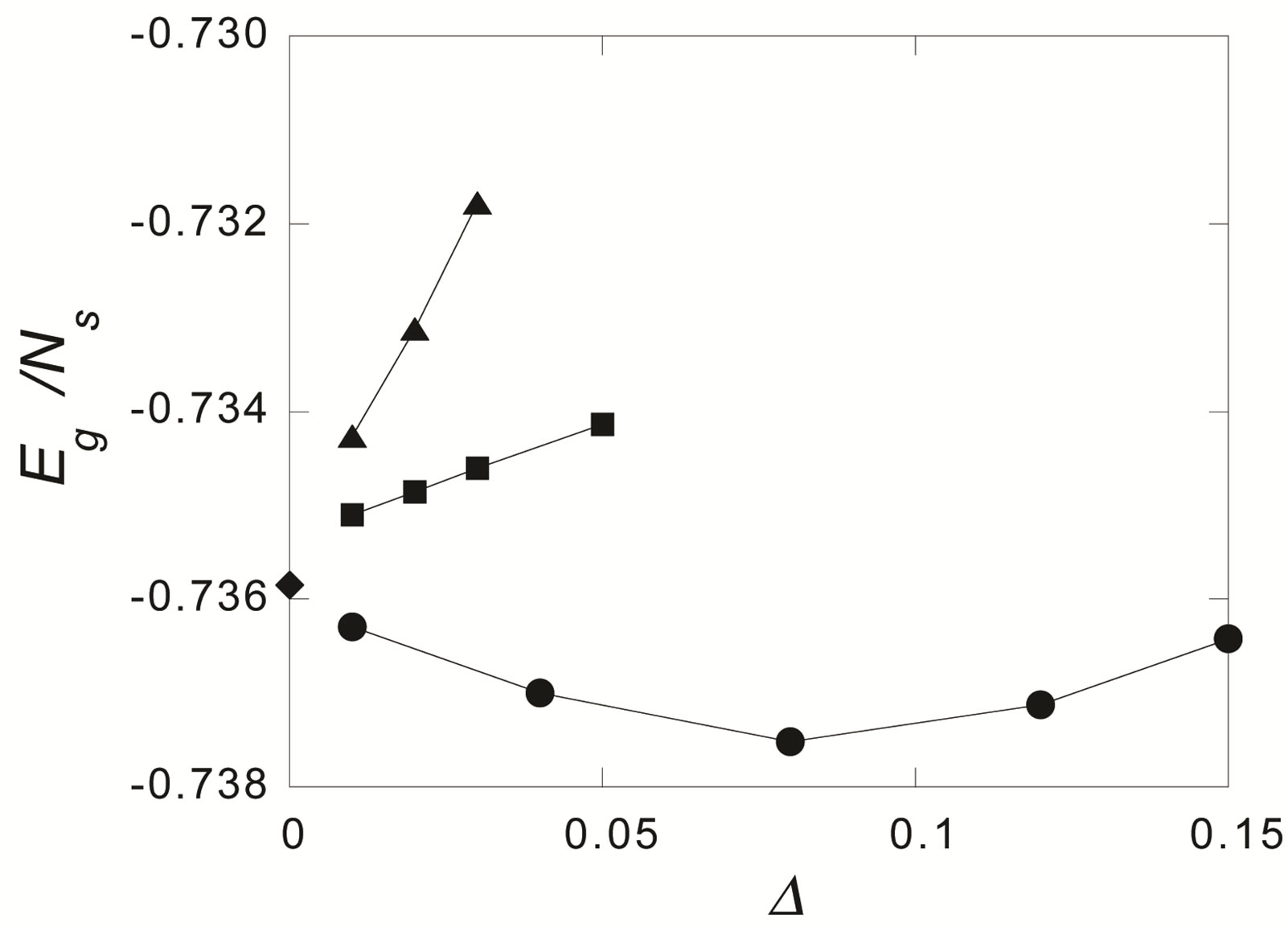
Figure 4. Ground state energy per site  for the 2D Hubbard model is plotted against
  for the case of 84 electrons on the 10 × 10 lattice with
  and
and . Solid curves are for the d-wave gap function. Squares and triangles are for the s*- and s-wave gap functions, respectively. The diamond shows the normal state value [46].
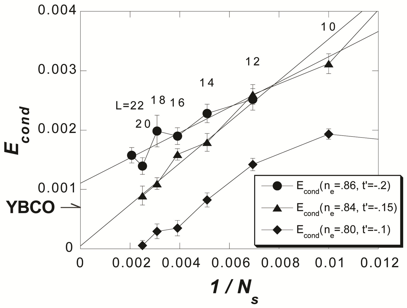
Figure 5. Energy gain per site in the SC state with reference to the normal state for the 2D Hubbard model is plotted as a function of . L is the length of the edge of the square lattice. YBCO attached to the vertical axis indicates the experimental value of the SC condensation energy for YBa2Cu3O4 [97].
clearly that the bulk limit remains finite when  and
and . When
 ,
,  and
and , the bulk-limit
  is
is , where t = 0.51 eV is used [98]. Thus the superconductivity is a real bulk property, not a spurious size effect. The value is remarkably close to experimental values 0.17 ~ 0.26 meV/site estimated from specific heat data [99,100] and 0.26 meV/site from the critical magnetic field
  [101] for optimally doped YBa2Cu3O4 (YBCO). This good agreement strongly indicates that the 2D Hubbard model includes essential ingredients for the superconductivity in the cuprates.
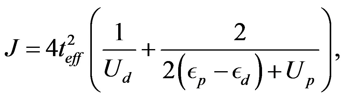
We just point out that the t-J model gives 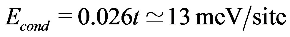 at
at  for J = 4 t2/U = 0.5 and
  [102]. This value is 50 times larger than the experimental values indicating a serious quantitative problem with this model. This means that the t-J model made from the leading two terms in the expansion in terms of
  of the canonical transformation of the Hubbard model should be treated with the higher-order terms in order to give a realistic SC condensation energy.
Here we show the SC condensation energy as a function of  in Figure 6. The condensation energy
  is increased as
  is increased as far as
 . In the strong coupling region
 , we obtain the large condensation energy.
3.3. Fermi Surface and Condensation Energy
Now let us consider the relationship between the Fermi surface structure and the strength of superconductivity. The experimental SC condensation energy for (La,Sr)2CuO4 (LSCO) is estimated at 0.029 meV/(Cu site) or 0.00008 in units of t which is much smaller than that

Figure 6. Energy gain per site in the SC state with reference to the normal state for the 2D Hubbard model as a function of the Coulomb repulsion U. The system is 10 × 10 with the electron number  and
and .
.
for YBCO. [103] The band parameter values of LSCO were estimated as  and
and  [104]. This set corresponds roughly to
 . The latter value is much larger than the above-mentioned experimental value for LSCO. However, the stripe-type SDW state coexists with superconductivity [105,106] and the SC part of the whole
  is much reduced. Therefore, such a coexistence allows us to qualitatively understand the SC
  in LSCO.
On the other hand, Tl2201  and Hg1201
  band calculations by Singh and Pickett [107] give very much deformed Fermi surfaces that can be fitted by large
  such as
 . For Tl2201, an Angular Magnetoresistance Oscillations (AMRO) work [108] gives information of the Fermi surface, which allows to get
  and
and . There is also an Angle-Resolved Photoemission Study (ARPES) [109], which provides similar values. In the case of Hg1201, there is an ARPES work [110], form which we obtain by fitting
  and
and . For such a deformed Fermi surface,
  in the bulk limit is reduced considerably. [111,112] Therefore, the SC
  calculated by VMC indicates that the Fermi surface of LSCO-type is more favorable for high
 . The lower
  in LSCO may be attributed to the coexistence with antiferromagnetism of stripe type.
3.4. Ladder Hubbard Model
The SC condensation energy in the bulk limit for the ladder Hubbard model has also been evaluated using the variational Monte Carlo method [54]. The Hamiltonian is given by the 1D two-chain Hubbard model: [51,52,55, 56,85,113-116]
 (29)
(29)
where 
 is the creation (annihilation) operator of an electron with spin
  at the
  th site along the
  th chain
 .
.  is the intrachain nearest-neighbor transfer and
  is the interchain nearest-neighbor transfer energy. The energy is measured in
  units. The energy minimum was given when the components of the gap function
  take finite values plotted in Figure 7 for the lattice of
  sites with 34 electrons imposing the periodic boundary condition [54]. Each component of
  was optimized for
  and
and . There are two characteristic features; one is that the components of the bonding and antibonding bands have opposite signs each other and second is that the absolute values of
  of the antibonding band
  is much larger than that of the bonding band
 . In order to reduce the computation cpu time,
 of each band was forced to take a fixed value specific to each band, i.e.
  for the bonding band and
  for the antibonding band. This drastically reduces the number of the variational parameters but still allows us to get a substantial value of the condensation energy.
  and
and  take opposite sign, which is similar to that of the
  gap function.
The energy gain  remains finite in the bulk limit when
 . The SC condensation energy per site in the bulk limit is plotted as a function of
  in Figure 8 [54]. The SC region derived from the SC condensation energy in the bulk limit is consistent with the results obtained from the density-matrix renormalization group [55,56] and the exact-diagonalization method [51,52,115]. The maximum value of
  is 0.0008 which is of the same order of magnitude as the maximum condensation energy obtained for the 2D Hubbard model [46].

Figure 7. The values of components of  for the twochain Hubbard model. All the values of
  of the bonding band
  and antibonding band
  correspond to the energy minimum for 20 × 2 lattice with 34 electrons. The parameters in the Hamiltonian are
  and
and  and the variational parameters are
  and
and  [54].
[54].
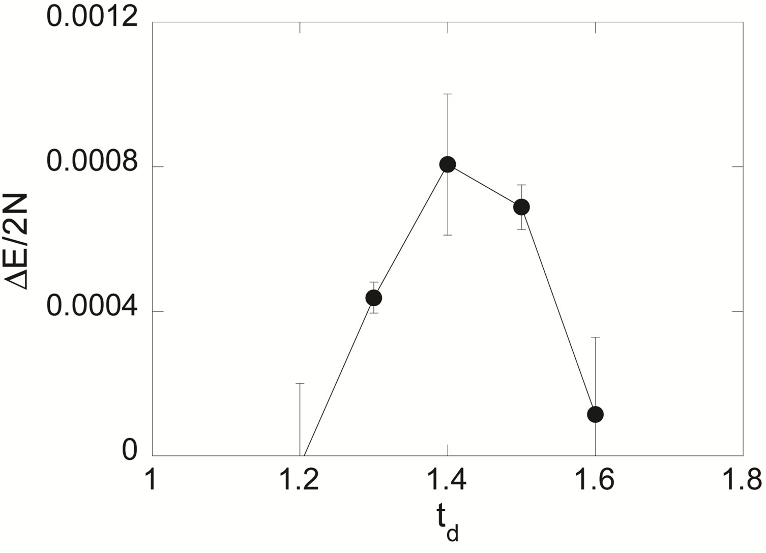
Figure 8.  dependence of the SC condensation energy
  for the two-chain Hubbard model in the bulk limit [54].
3.5. Condensation Energy in the d-p Model
The SC energy gain for the d-p model, namely, threeband Hubbard model in Equation (4) has also been evaluated using the variational Monte Carlo method. For the three-band model the wave functions are written as
 (30)
(30)
 (31)
(31)
where  is the linear combination of
 ,
,  and
and  constructed to express the operator for the lowest band (in the hole picture) or the highest band (in the electron picture) of the non-interacting Hamiltonian. The numerical calculations have been done in the hole picture. The Gutzwiller parameter
 , effective level difference
 , chemical potential
  and superconducting order parameter
  are the variational parameters.
The similar results to the single-band Hubbard model were obtained as shown in Figure 9 for ,
,  and
and  in
in  units where the calculations were performed in the hole picture [24]. The SC condensation energy for the three-band model is
  meV per site in the optimally doped region. We set
  as estimated in Table 1. There is a tendency that
  increases as
  increases which is plotted in Figure 10. This tendency is not, however, in accordance with NQR (nuclear quadrupole resonance) study on cuprates. [117] We think that the NQR experiments indicate an importance of the Coulomb interaction on oxygen sites. This will be discussed in Section 3.11.
3.6. Antiferromagnetic State
When the density of doped holes is zero or small, the 2D single-band or three-band Hubbard model takes an antiferromganetic state as its ground state. The magnetic

Figure 9. Ground-state energy per site as a function of  with the d-wave gap function for the three-band Hubbard model. The size of lattice is 6 × 6. Parameters are
 ,
,  and
and  in units of
 . The doping rate is
  for (a) and
  for (b). Squares denote the energies for the normal-state wave function [24].
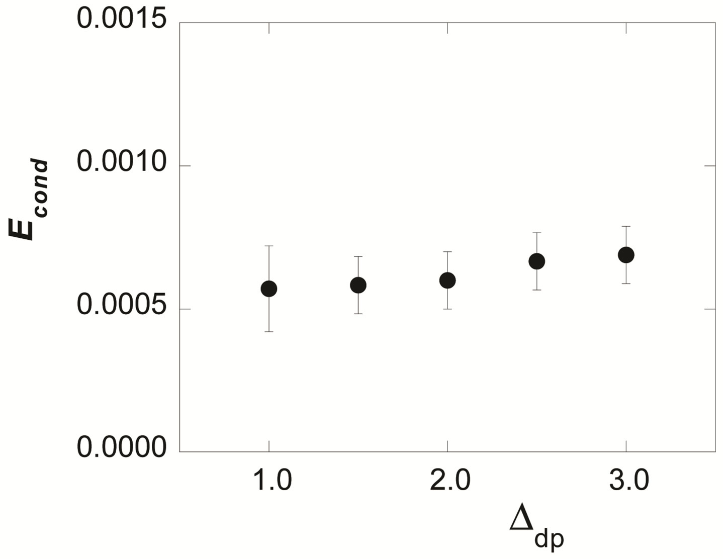
Figure 10. Energy gain per site in the SC state as a function of the level difference  for the three-band Hubbard model with
  and
and  [24]. The size of lattice is 6 × 6 sites.
order is destroyed and superconductivity appears with the increase of doped hole density. The transition between the d-wave SC and the uniform SDW states has been investigated by computing the energy of the SDW state by using the variational Monte Carlo method. The trial SDW wave function is written as
 (32)
(32)
 (33)
(33)
 (34)
(34)
 (35)
(35)
 (36)
(36)
Summation over  and
and  in Equation (33) is performed over the filled k-points, as in the calculation of the normal state energy.
  is the SDW wave vector given by
  and
and  is the SDW potential amplitude.
As shown in Figure 11, the energy gain per site in the SDW state rises very sharply from  for
for  [46]. At
  it is slightly larger than that in the SC state, and at
  there is no more stable SDW state. Thus the boundary between the SDW and the SC states is given at
 . The results of the bulk limit calculations indicate that the energy gain in the SC state at
  takes the extremely small value and the value at
  vanishes as
 . Hence the pure d-wave SC state possibly exists near the boundary at
 , but the region of pure SC state is very restricted.
Let us turn to the three-band model. We show the antiferromagnetic-paramagnetic boundary for  and
and  in the plane of
  and the hole density in Figure 12 where AF denotes the antiferromagnetic region [47]. The value
  is taken from the estimations by cluster calculations [89-91]. The phase boundary in the region of small
  is drawn from an extrapolation. For the intermediate values of
 ,
,
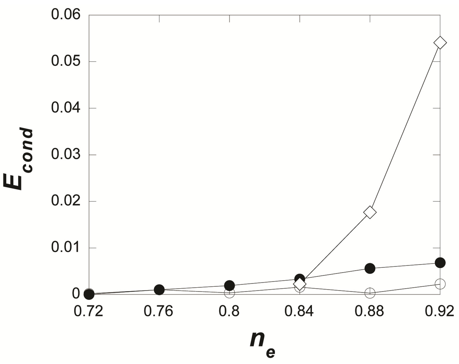
Figure 11. Energy gain per site in the SDW state (diamonds) against electron density for  and the energy gain in the SC state for
  (open circles) and
 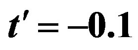 (solid circles). The model is the 2D Hubbard model on 10 × 10 lattice [46].
Figure 12. Antiferromagnetic region in the plane of U and the hole density for  and
and .
.
the antiferromagnetic long-range ordering exists up to about 20 percent doping. Thus the similar features are observed compared to the single-band Hubbard model.
Since the three-band Hubbard model contains several parameters, we must examine the parameter dependence of the energy of SDW state. The energy gain  in the SDW state is shown in Figure 13 as a function of doping ratio for several values of
 .
.  increases as
  increases as expected. In Figure 14
  - and
- and  -dependencies of
  are presented. The SDW phase extends up to 30 percent doping when
  is large. It follows from the calculations that the SDW region will be reduced if
  and
and  decrease.
From the calculations for the SDW wave functions, we should set  and
and  small so that the SDW phase does not occupy a huge region near half-filling. In Figures 15 and 16, we show energy gains for both the SDW and SC states for
 ,
,  ,
,  and
and , where the right hand side and left hand side indicate the hole-doped and electron-doped case, respectively. Solid symbols indicate the results for
  and open symbols for
 . For this set of parameters the SDW region extends up to 20 percent doping and the pure d-wave phase exists outside of the SDW phase. The d-wave phase may be possibly identified with superconducting phase in the overdoped region in the high-
 superconductors.
3.7. Stripes and Its Coexistence with Superconductivity
Incommensurate magnetic and charge peaks have been observed from the elastic neutron-scattering experiments in the underdoped region of the Nd-doped La2–x–yNdySrxCuO4 [118] (Figure 17). Recent neutron experiments have also revealed the incommensurate spin structures [119-123]. Rapid decrease of the Hall resistivity in this region suggests that the electric con-
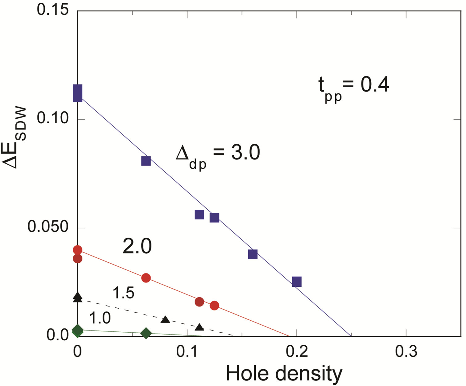
Figure 13. Energy gain per site  in the SDW state as a function of hole density
  for the threeband Hubbard model. Parameters are
  and
and  in
in  units. From the top,
  , 2, 1.5 and 1. The results are for 6 × 6, 8 × 8, 10 × 10 and 16 × 12 systems. Antiperiodic and periodic boundary conditions are imposed in xand y-direction, respectively. Monte Carlo statistical errors are smaller than the size of symbols. Curves are a guide to the eye [24].

Figure 14. Uniform SDW energy gain per site with reference to the normal-state energy as a function of the hole density for the three-band Hubbard model. Data are from 8 × 8, 10 × 10, 12 × 12 and 16 × 12 systems for . For solid symbols
  (circles),
  (squares),
  (triangles) and
  (diamonds) for
 . For open symbols
  and
and , and for open squares with slash
  and
and . The lines are a guide to the eye. The Monte Carlo statistical errors are smaller than the size of symbols [47].
duction is approximately one dimensional [124]. The angle-resolved photo-emission spectroscopy measurements also suggested a formation of two sets of onedimensional Fermi surface [125]. Then it has been proposed that these results might be understood in the framework of the stripe state where holes are doped in the domain wall between the undoped spin-density-wave

Figure 15. Condensation energy per site as a function of hole density for the three-band Hubbard model where ,
,  and
and . Circles and squares denote the energy gain per site with reference to the normal-state energy for d-wave, ext-s wave and SDW states, respectively. For extremely small doping rate, the extended s-wave state is more favorable than the d-wave state. Solid symbols are for 8 × 8 and open symbols are for 6 × 6. Curves are a guide to the eye.
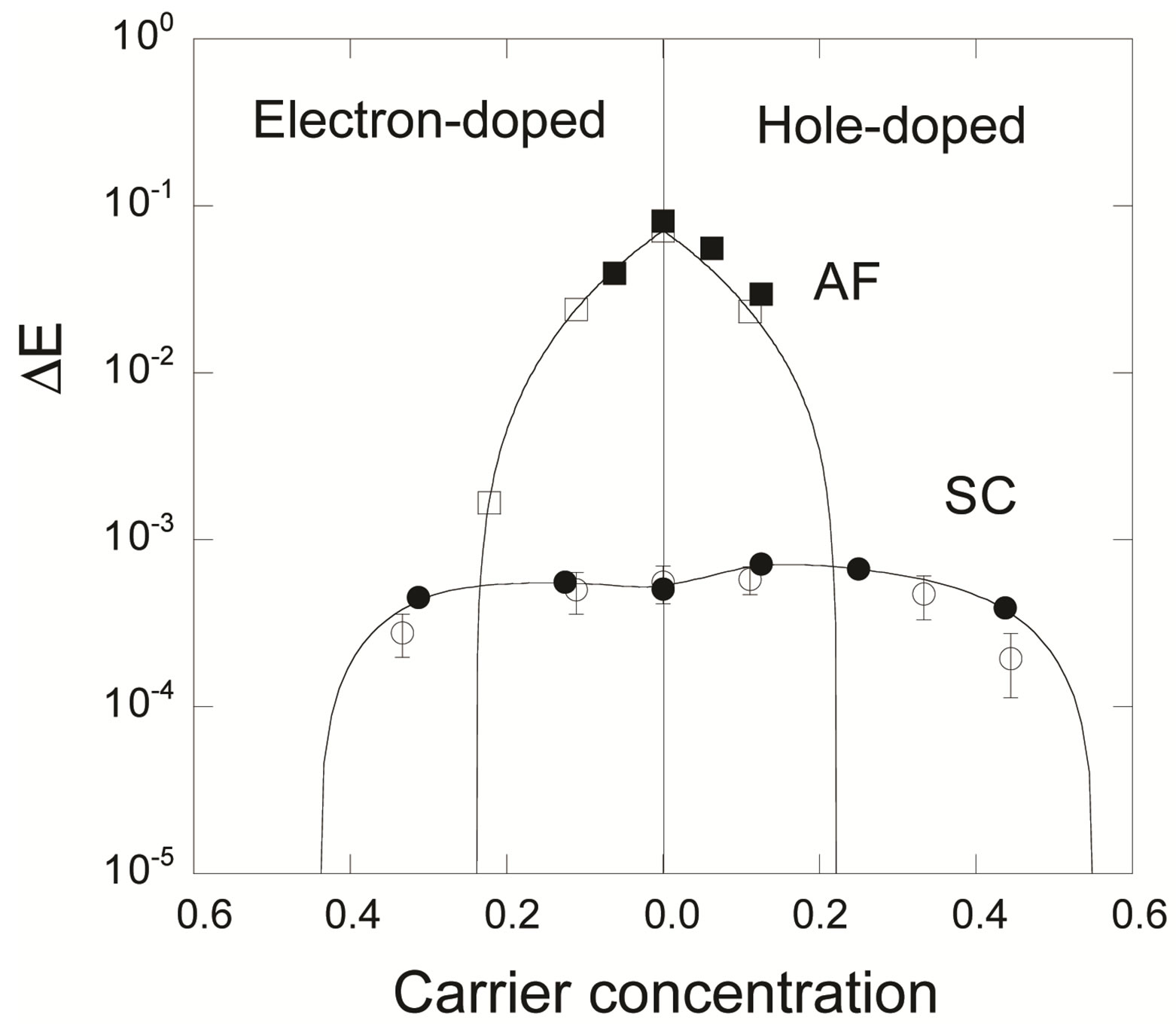
Figure 16. Condensation energy per site as a function of hole density for the three-band Hubbard model where ,
,  and
and . Circles and squares denote the energy gain per site with reference to the normal-state energy for d-wave and SDW states, respectively. Solid symbols are for 8 × 8 and open symbols are for 6 × 6. Curves are a guide to the eye.
domains. This state is a kind of incommensurate SDW state. It was also shown that the incommensurability is proportional to the hole density in the low-doping region in which the hole number per stripe is half of the site number along one stripe [118,120]. A static magnetically ordered phase has been observed by  SR over a wide range of SC phase for
  in La2–xSrxCuO4 (LSCO) [126]. Thus the possibility of superconductivity that occurs in the stripe state is a subject of great interest [127-130]. The incommensurate magnetic scattering spots around
  were observed in the SC phase in the range of
  in the elastic and inelastic neutron-scattering experiments with LSCO [127,128,130]. The hole dependence of the incommensurability and the configuration of the spots around the Bragg spot in the SC phase indicated the vertical stripe. The neutronscattering experiments have also revealed that a diagonal spin modulation occurs across the insulating spin-glass phase in La2–xSrxCuO4 for
 , where a one-dimensional modulation is rotated by 45 degrees from the stripe in the SC phase. The incommensurability
  versus hole density is shown in Figure 18 schematically [129,130]. The diagonal stripe changes into the vertical stripe across the boundary between the insulating and SC phase.
Let us investigate the doped system from the point of modulated spin structures [131-141]. The stripe SDW state has been studied theoretically by using the meanfiled theory [132-136]. They found that the stripe state appears when an incommensurate nesting becomes
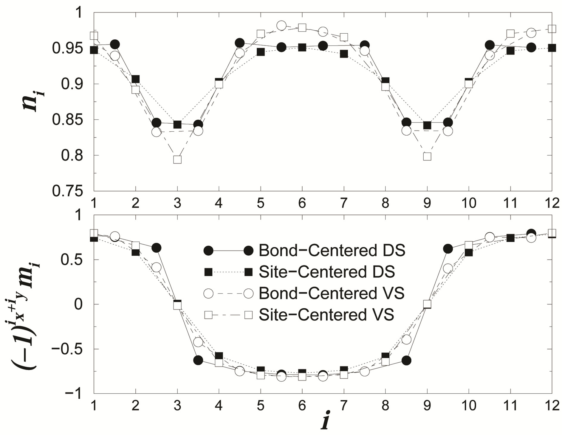
Figure 17. Charge and spin density as a function of the distance for a striped state [50].
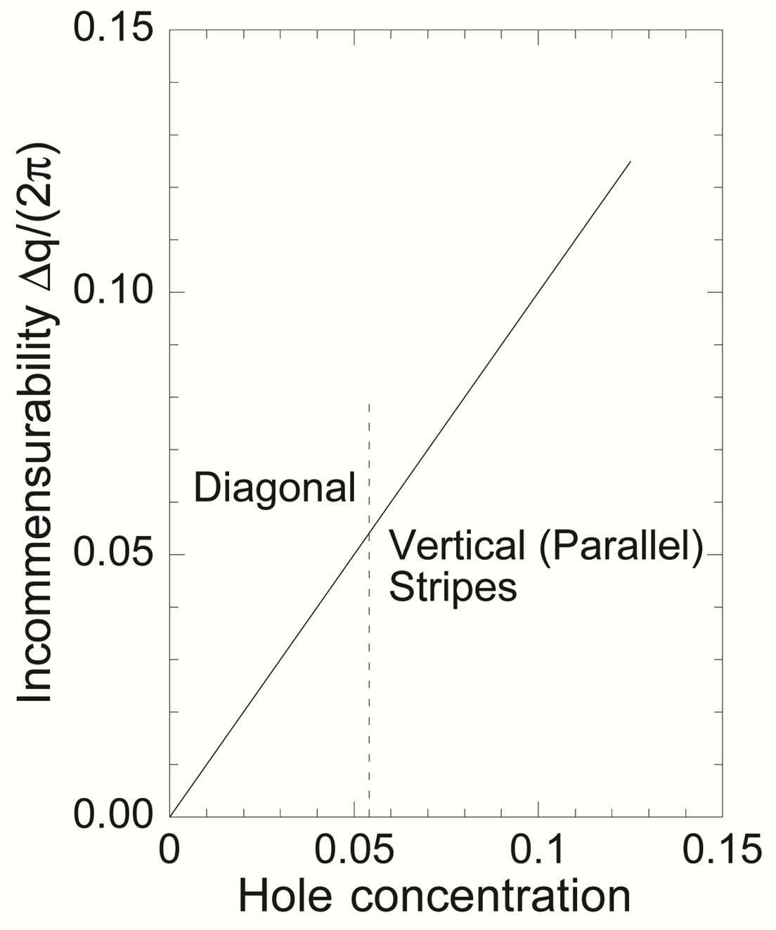
Figure 18. Schematic illustration of the incommensurability versus hole density.
favorable in the hole-doped 2D Hubbard model. When the electron correlation correlation is strong or intermediate, it was shown that the stripe state is more stable than the commensurate spin-density-wave state with the wave vector  in the ground state of the 2D Hubbard model by using the variational Monte Carlo method [131]. It has also been confirmed by the same means that the stripe states are stabilized in the d-p model [48]. The purpose of this section is to examine whether the superconductivity can coexist with static stripes in the 2D Hubbard model in a wider doping region and investigate the doping dependence of the coexisting state.
We consider the 2D Hubbard model on a square lattice. We calculate the variational energy in the coexistent state that is defined by
 (37)
(37)
where  is a mean-field wave function. The effective mean-field Hamiltonian for the coexisting state is [105] represented by
 (38)
(38)
where the diagonal terms describe the incommensurate spin-density wave state:
 (39)
(39)
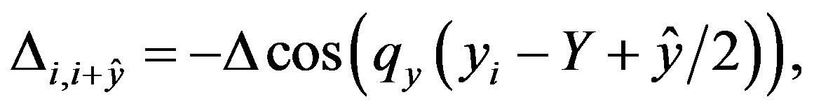
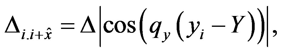
where  is the chemical potential. The vertical stripe state is represented by the charge density
  and the spin density
  that are spatially modulated as
 (40)
(40)
 (41)
(41)
where  denotes the position of vertical stripes. The amplitude
  is fixed by
 . The off-diagonal terms in Equation (38) are defined in terms of the d-wave SC gap as
 (42)
(42)
where ,
,  (unit vectors). We consider two types of the spatially inhomogeneous superconductivity: anti-phase and in-phase defined as
 (43)
(43)
 (44)
(44)
and
 (45)
(45)
 (46)
(46)
respectively. Here,  and
and  is a incommensurability given by the stripe’s periodicity in the y direction with regard to the spin. The anti-phase (inphase) means that the sign if the superconducting gap is (is not) changed between nearest domain walls.
The wave function  is made from the solution of the Bogoliubov-de Gennes equation represented by
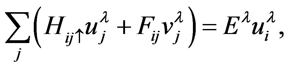 (47)
(47)
 (48)
(48)
The Bogoliubov quasiparticle operators are written in the form
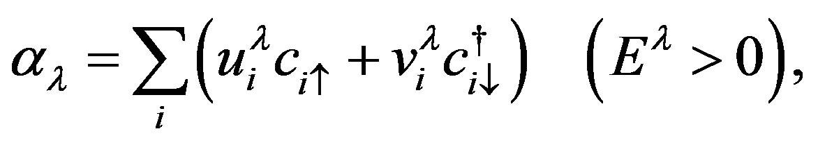 (49)
(49)
 (50)
(50)
Then the coexistence wave function is written as [105,142]
 (51)
(51)
for constants  and
and . The calculations are performed for the wave function
 . The variational parameters are
 ,
,  ,
,  ,
,  and
and . The system parameters were chosen as
  and
and  suitable for cuprate superconductors. It has been shown that the “anti-phase” configuration is more stable than the “in-phase” one [105].
Here, the system parameters are  and
and . We use the periodic boundary condition in the x-direction and anti-periodic one in the y-direction. In Figure 19, we show the total energy of the coexistent state,
  , as a function of the SC gap
  for the cases of anti-phase and in-phase. The SC condensation energy
  is estimated as 0.0008 t per site at the hole density 0.125 on the
  lattice with periodic boundary condition in x-direction and antiperiodic one in y-direction.
  in the coexistence state is defined as the decrease of energy due to finite
 . If we use
 , this is evaluated as
 . The SC condensation energy per site is shown as a function of hole density in Figure 20. One finds that
  in the stripe state decreases as the hole density decreases. This tendency is reasonable since the SC order is weakened in the domain of the incommensurate SDW because of the vanishingly small carrier concentration contributing the superconductivity in this domain. This behavior is consistent with the SC condensation energy estimated from the specific heat measurements [143].
There is a large renormalization of the Fermi surface due to the correlation effect in the striped state [144]. We considered the next-nearest transfer  in the trial function as a variational parameter
 . In Figure 21,
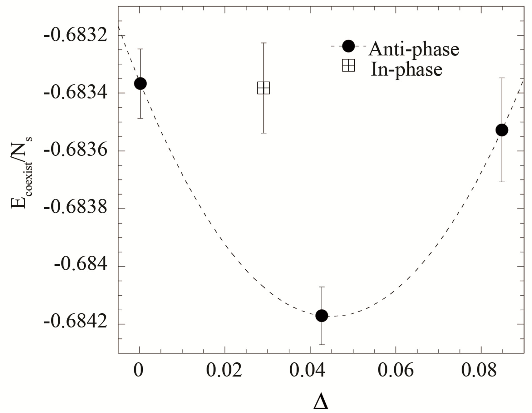
Figure 19. Coexistent state energy per site  versus
  for the case of 84 electrons on 12 × 8 sites with
  and
and . Here the vertical stripe state has 8-lattice periodicity for the hole density
 . Only
  for the optimized gap is plotted for the in-phase superconductivity.
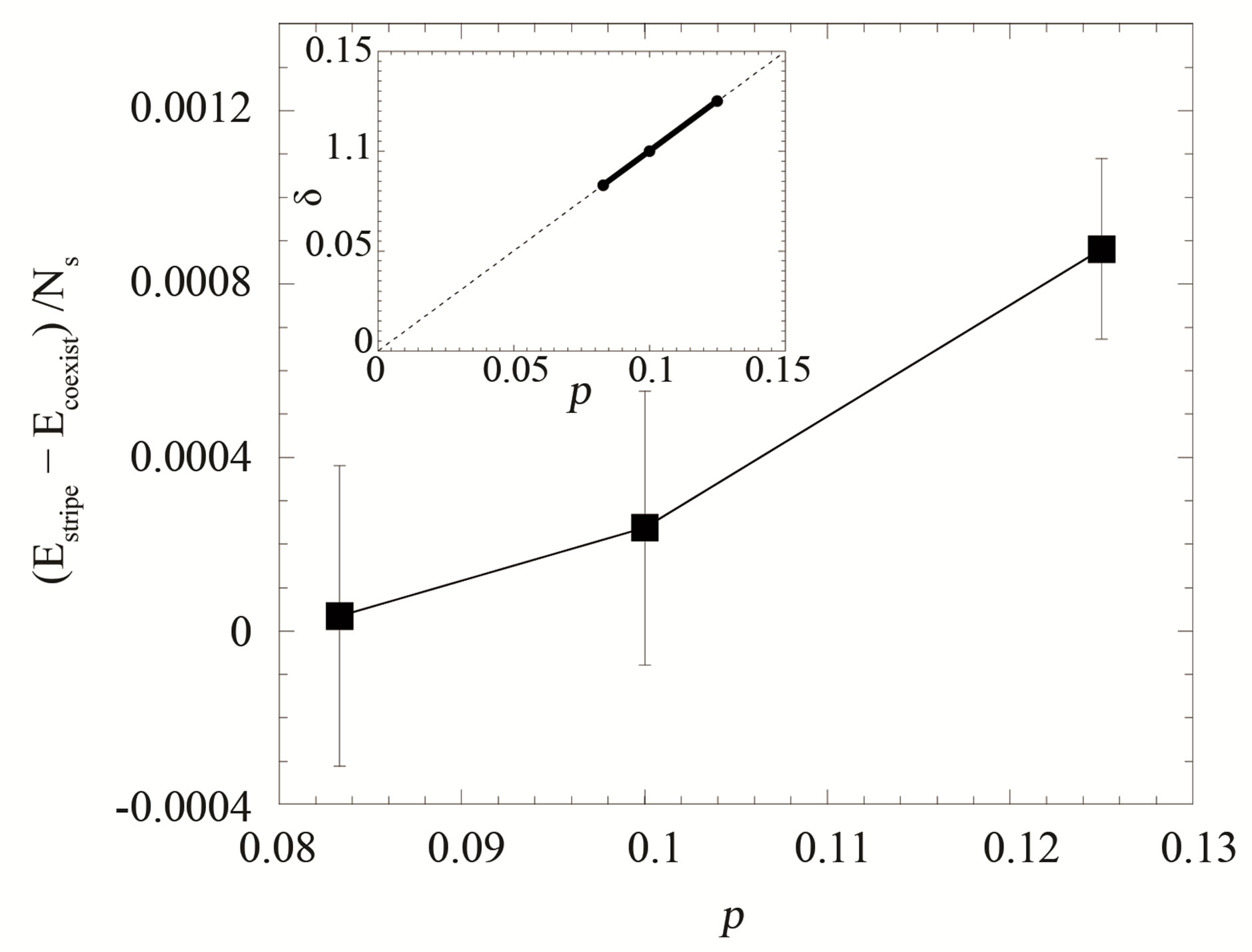
Figure 20. Superconducting condensation energy per site in the coexistence state as a function of the hole density , 0.10 and 0.125. The model is the single-band Hubbard Hamiltonian with
 . The stripe interval is preserved constant. The inset shows the hole dependence of the incommensurability in the coexistent state [105].

Figure 21. Optimized effective second neighbor transfer energy  as a function of
 . The system is a 16 × 16 lattice with
  and the electron density 0.875.
optimized values of  for the striped state are shown as a function of
 . The
. The  increases as
  increases. We also mention that the optimized
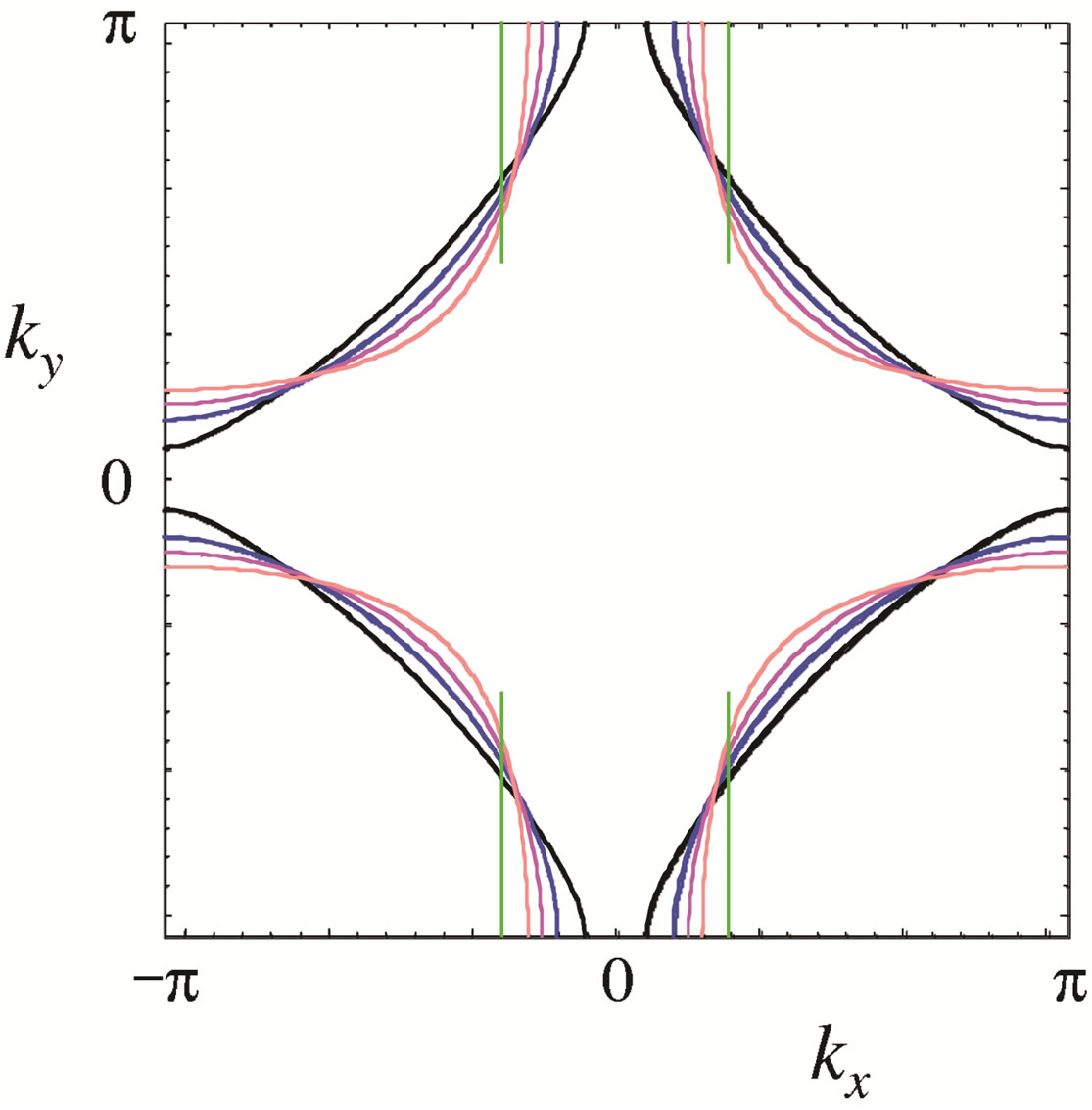
  almost vanishes. The renormalized Fermi surface of
 ,
,  and
and  are plotted in Figure 22. The system is a
  lattice with
  and the electron density 0.875. As
  is incresed, the Fermi surface is more deformed. We show the the gradient of the momentum distribution function,
  , calculated in the optimized stripe state in Figure 23. The brighter areas coincide with the renormalized Fermi surface with
  and
and  for
for .
.
The calculations for the three-band Hubbard model has also been done taking into account the coexistence of stripes and SC [15,106]. The energy of antiferromagnetic state would be lowered further if we consider the incommensurate spin correlation in the wave function. The phase diagram in Figure 24 presents the region of stable AF phase in the plane of  and
and . For large
 , we have the region of the AF state with an eight-lattice periodicity in accordance with the results of neutron-scattering measurements [118,123]. The energy at
  is shown in Figure 25 where the 4-lattice stripe state has higher energy than that for 8-lattice stripe for all the values of
 .
.
The Bogoliubov-de Gennes equation is extended to the case of three orbitals ,
,  and
and .
.  and
and  are now
  matrices. The energy of the state with double order parameters
  and
and  is shown in Figure 26 on the
  lattice at the doping rate 1/8. The SC condensation energy per site is evaluated as
  for
for ,
,  and
and . If we use
  [89-91], we obtain
 which is slightly smaller than and close to the value obtained for the single-band Hubbard model. We show the size dependence of the SC condensation
 ,
,  and
and . The system is the same as that in
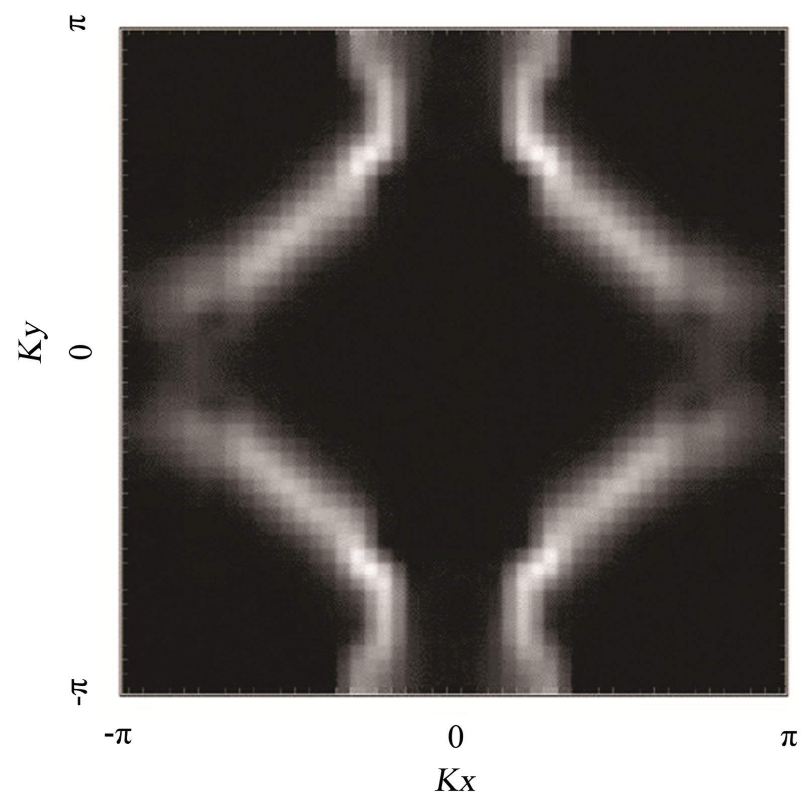
Figure 23. Contour plot of  measured for the projected stripe state on 24 × 24 lattice with
 . The electron density is 0.875.
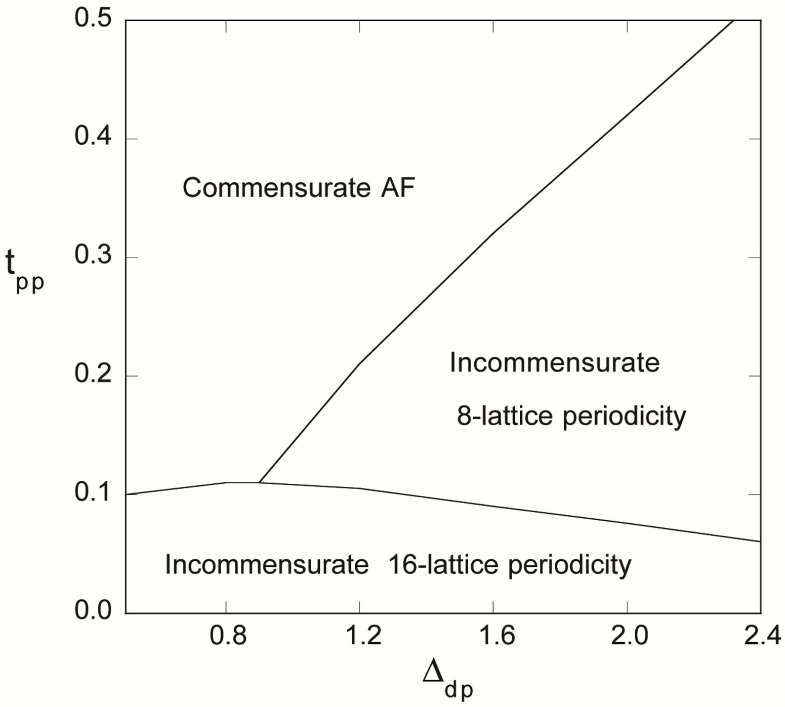
Figure 24. Phase diagram of stable antiferromagnetic state in the plane of  and
and  obtained for 16 × 4 lattice.
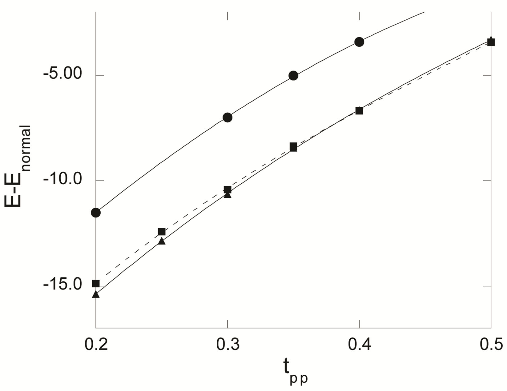
Figure 25. Energy as a function of  for 16 × 16 square lattice at
 . Circles, triangles and squares denote the energy for 4-lattice stripes, 8-lattice stripes, and commensurate SDW, respectively, where n-lattice stripe is the incommensurate state with one stripe per n ladders. The boundary conditions are antiperiodic in x-direction and periodic in y-direction [47,106].
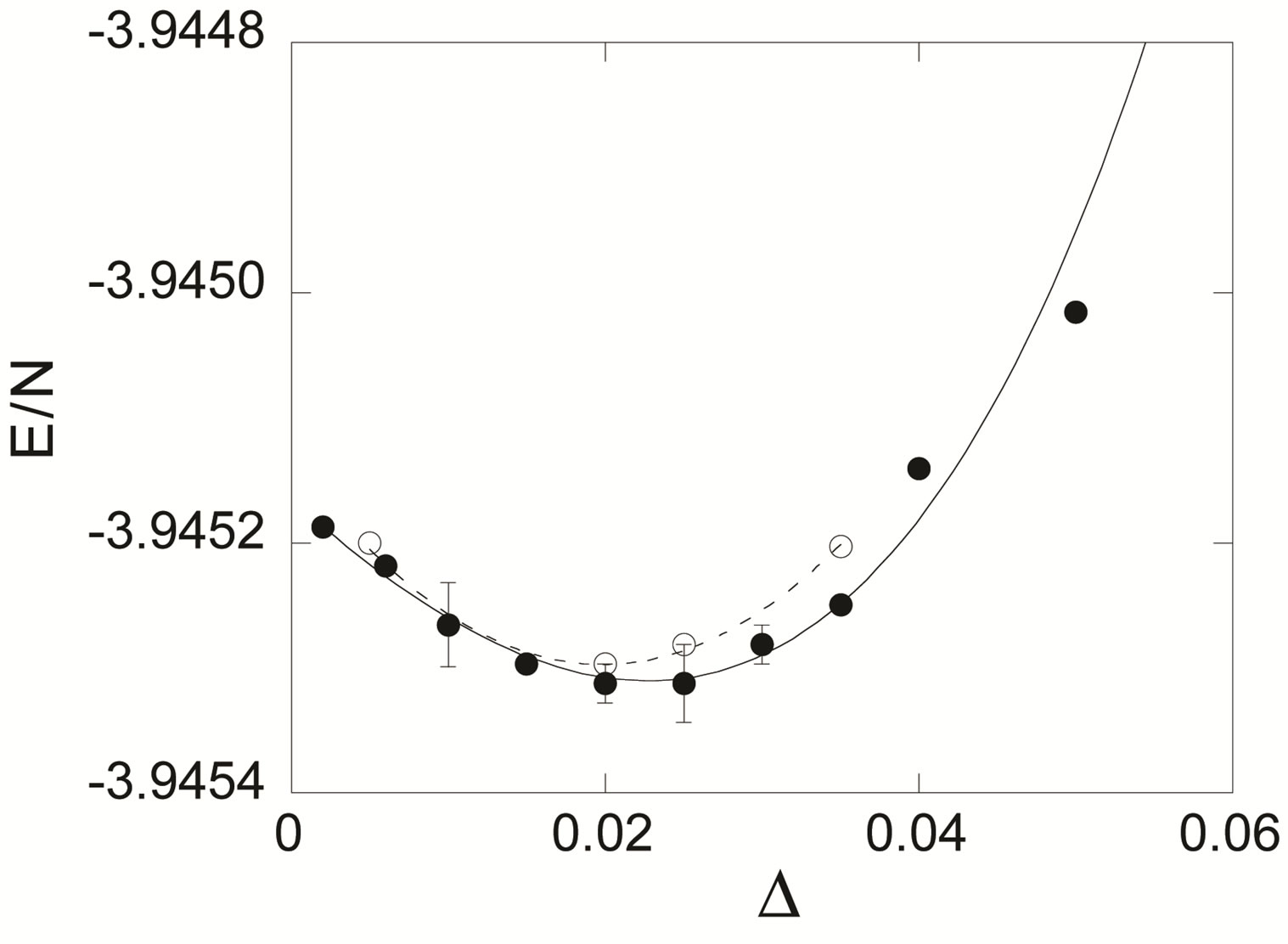
Figure 26. Energy of the coexistent state as a function of the SC order parameter for  on 16 × 4 lattice. We assume the incommensurate antiferromagnetic order (stripe). Parameters are
 ,
,  ,
,  and
and  in
in  units. For solid circles the SC gap function is taken as
 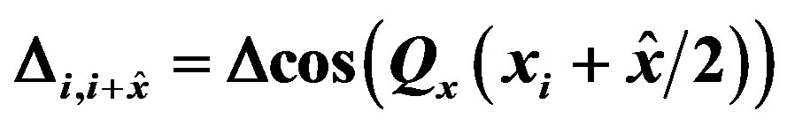 and
and  , while for the open circles
  and
and .
.  .
.
energy for , 0.125 0.08333 and 0.0625 in Figure 27. We set the parameters as
  and
and  in
in  units, which is reasonable from the viewpoint of the density of states and is remarkably in accordance with cluster estimations [89-91], and also in the region of eight-lattice periodicity at
 . We have carried out the Monte Carlo calculations up to
  sites (768 atoms in total). In the overdoped region in the range of
 , we have the uniform d-wave pairing state as the ground state. The periodicity of spatial variation increases as the doping rate
  decreases proportional to
 . In the figure we have the 12-lattice periodicity at
  and 16-lattice periodicity at
 . For
. For , 0.125 and 0.08333, the results strongly suggest a finite condensation energy in the bulk limit. The SC condensation energy obtained on the basis of specific heat measurements agrees well with the variational Monte Carlo computations [99]. In general, the Monte Carlo statistical errors are much larger than those for the single-band Hubbard model. The large number of Monte Carlo steps (more than
 ) is required to get convergent expectation values for each set of parameters.
In Figure 28 the order parameters  and
and 
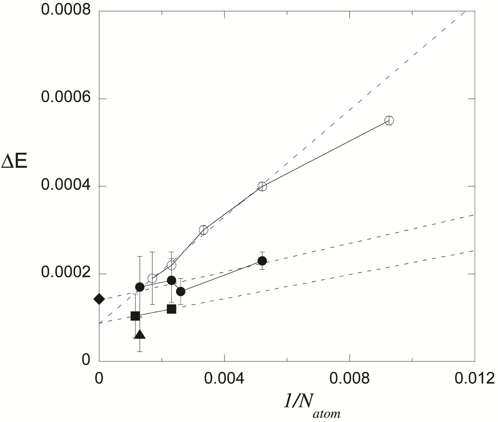
Figure 27. Energy gain due to the SC order parameter as a function of the system size . Parameters are
 ,
,  ,
,  and
and . The open circle is for the simple d-wave pairing at the hole density
 . The solid symbols indicate the energy gain of the coexistent state; the solid circle is at
  , the solid square is at
  and the solid triangle is at
 . The diamond shows the SC condensation energy obtained on the basis of specific heat measurements [99].

Figure 28. Phase diagram of the d-p model based on the Gutzwiller wave function [106].
were evaluated using the formula  where
where  is the density of states. Here we have set
  since
since  is estimated as
to 3  for optimally doped YBCO using
 [100]. The phase diagram is consistent with the recently reported phase diagram for layered cuprates [145].
3.8. Diagonal Stripe States in the Light-Doping Region
Here we examine whether the relationship  holds in the lower doping region or not, and whether the diagonal stripe state is obtained in the further lower doping region [50]. The elastic neutron scattering experiments of LSCO in the light-doping region,
  , revealed that the position of incommensurate magnetic peaks changed from
  to
to  as
as  becomes less than 0.06 [129,130]. This means that the stripe direction rotates by 45 degrees to become diagonal at this transition. In the diagonal stripe states, the magnetic peaks are observed to keep a relation
  that holds in the vertical stripe state in the low doping region.
In Figure 29, we show the incommensurability of the most stable stripe state as a function of . Open squares and triangles are values for diagonal and vertical incommensurate SDW’s obtained in the elastic neutron scattering experiments on LSCO, respectively. Solid squares and triangles show our results for the diagonal and vertical stripes, respectively. These results are in a good agreement with experimental data. We also found that the phase boundary
  between the diagonal and vertical stripe states lies at or above 0.0625 in the
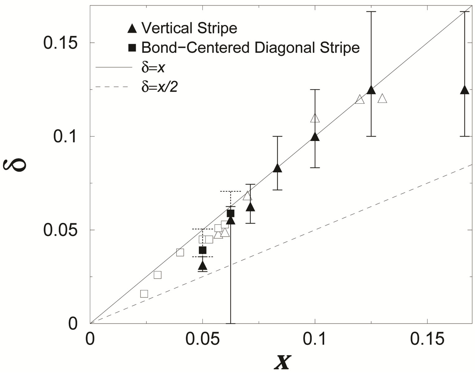
Figure 29. Incommensurability  as a function of the hole density x for
  and
and  [50]. The numerical results for the vertical and the bond-centered diagonal stripe state are represented by solid triangles and square symbols, respectively. Open triangles and squares show the results of the vertical and diagonal incommensurate SDW order observed from neutron scattering measurements, respectively [131].
case of  and
and . The following factors may give rise to slight changes of the phase boundary
 : the diagonal stripe state may be stabilized in the low-temperature-orthorhombic (LTO) phase in LSCO. The diagonal stripe state is probably stabilized further by forming a line along larger next-nearest hopping direction due to the anisotropic
  generated by the Cu-O buckling in the LTO phase.
3.9. Checkerboard States
A checkerboard-like density modulation with a roughly  period (
 is a lattice constant) has also been observed by scanning tunneling microscopy (STM) experiments in Bi2Sr2CaCu2O8+d, [146] Bi2Sr2–xLaxCuO6+d, [147] and Ca2–xNaxCuO2Cl2 (Na-CCOC) [148]. It is important to clarify whether these inhomogeneous states can be understood within the framework of strongly correlated electrons.
Possible several electronic checkerboard states have been proposed theoretically [134,149,150]. The charge density  and spin density
  are spatially modulated as
 (52)
(52)
 (53)
(53)
where  and
and  are variational parameters. The striped incommensurate spin-density wave state (ISDW) is defined by a single Q vector. On the other hand, the checkerboard ISDW state is described by the double-Q set; for example, vertical wave vectors
  and
and  describe a spin vertical checkerboard state, where two diagonal domain walls are orthogonal. Diagonal wave vectors
  and
and  lead to a spin diagonal checkerboard state with a
  -period. The hole density forms the charge vertical checkerboard pattern with vertical wave vectors
  and
and  in which the hole density is maximal on the crossing point of magnetic domain walls in the spin diagonal checkerboard state. If
  is assumed, the charge modulation pattern is consistent with the
  charge structure observed in STM experiments.
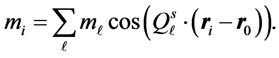
We found that the coexistent state of bond-centered four-period diagonal and vertical spin-checkerboard structure characterized by a multi-Q set is stabilized and composed of  period checkerboard spin modulation. [151] In Figure 30(a), we show the condensation energies of some heterogeneous states,
  , with fixing the transfer energies
  and
and  suitable for Bi-2212. The system is a
  lattice with the electron-filling

Figure 30. (a) Condensation energies of inhomogeneous states with the bond-centered magnetic domain wall. The system is a 16 × 16 lattice with ,
,  , and
, and  for the case of
 . The static error bars are smaller than the size of symbols; (b) Expectation value of the spin density
  measured in the four-period spin-DCVC solution. The length of arrows is proportional to the spin density.
 . The energy of the normal state
  is calculated by adopting
 . In our calculations, the condensation energies of both bondcentered stripe and checkerboard states are always larger than those of site-centered stripe and checkerboard states. The vertical stripe state is not suitable in this parameter set since this state is only stabilized with the LSCO-type band. The four-period spin-diagonal checkerboard (DC) state is significantly more stable than the eight-period spin-DC state. We found that the coexistent state of the bond-centered four-period spin-DC and four-period spin-vertical checkerboard (VC) with
  is most stable, as shown in Figure 30(a). The measured expectation value of the spin density is shown in Figure 30(b).
3.10. Improved Gutzwiller Function
We have presented the results based on the Gutzwiller functions for the normal state, SDW state and BCS state. We must consider a method to go beyond the Gutzwiller function-based Monte Carlo method. One method to achieve this purpose is to multiply the Jastrow correlation operators to take into account the intersite correlations. The simplest possible candidate is an introduction of the diagonal intersite correlation factor [152]:
 (54)
(54)
for the variational parameter . We have investigated the 2D Hubbard model by using the JastrowGutzwiller function [111]. The ground-state energy is lowered considerably by considering the intersite correlations such as nearest neighbor and next nearest neighbor spin and charge correlations.
Here we consider the method to improve the wave functions by an off-diagonal Jastrow correlation operators [94,95,153]. The off-diagonal correlation factors are more effective to lower the ground state energy in 2D systems. Let us consider the wave functions  defined in the following way: [95]
 (55)
(55)
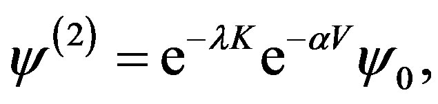 (56)
(56)
 (57)
(57)

 (58)
(58)
and so on, where  denotes the kinetic part of the Hamiltonian
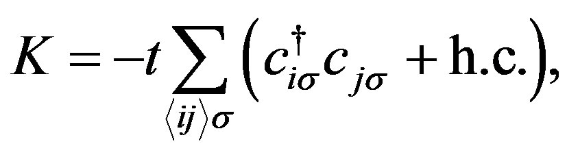 (59)
(59)
and  denotes the on-site Coulomb interaction.
 ,
,  ,
,  ,
,  ,
,  and
and  are variational parameters. It is considered that
  approaches the true ground state wave function as
  grows larger since the ground state wave function is written as
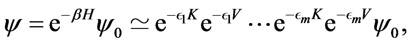 (60)
(60)
for large  and small
 . If we can extrapolate the expectation values from the data for
 , we can evaluate correct expectation values.
The computations are performed by using the discrete Hubbard-Stratonovich transformation as described in Section 3.1. In the evaluation of the expectation values we generate the Monte Carlo samples by the importance sampling [95] with the weight function  where
where
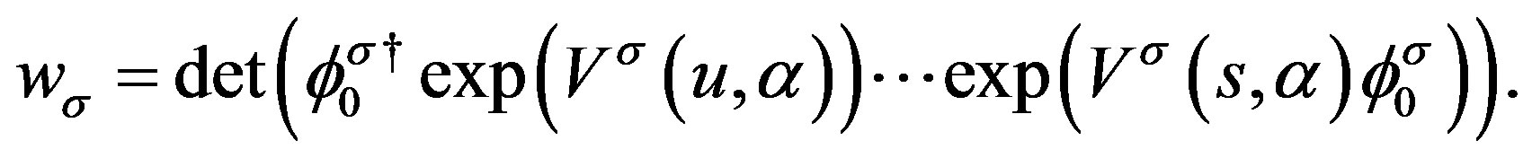 (61)
(61)
Since the Monte Carlo samplings are generated with the weight , the expectation values are calculated with the sign of
  in the summation over the generated samples. In our calculations the negative sign problem has become less serious due to the variational treatment, although we encounter the inevitable negative sign problem in the standard projector Monte Carlo approaches [154].
In Figure 31 the energy is shown as a function of  where the SDW and normal states are chosen as the initial state
 . The extrapolated values for different initial states coincide with each other within Monte Carlo statistical errors. The energy expectation values as a function of
  for
for  square lattice are presented in Figure 32 for
 ,
,  ,
, . The extrapolated curve is shown by the solid curve and the results obtained by the quantum Monte Carlo simulation (QMC) [28] are also shown as a reference. A good agreement between two calculations support the method although the QMC gives slightly higher energy for
 .
.
One can formulate an approach to consider the BCS function with correlation operators. [96] For this end the electron-hole transformation is introduced for the down spin and the up-spin electrons are unaltered [155]. We show the energy versus  in Figure 33 for
  and
and . From an extrapolation to the limit
 , both formulations predict the same limiting value for the energy. The energy is lowered considerably due to the
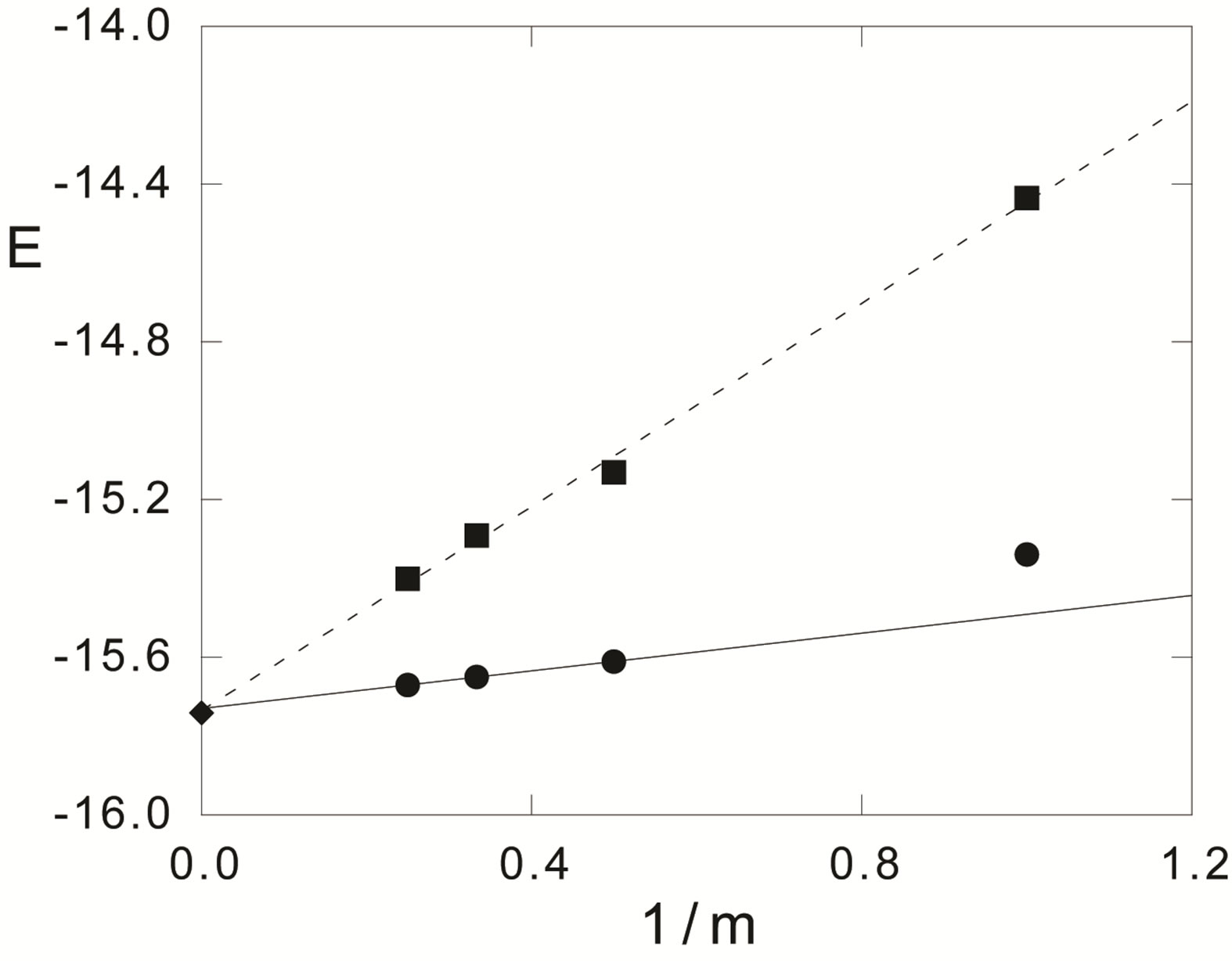
Figure 31. Energy as a function of  for the single-band Hubbard model for
  and
and  on the lattice of 4 × 4 sites. For the upper and lower curves, the initial wave function
  is the Fermi sea and SDW state, respectively. The diamond indicates the exact value obtained from the diagonalization [95].
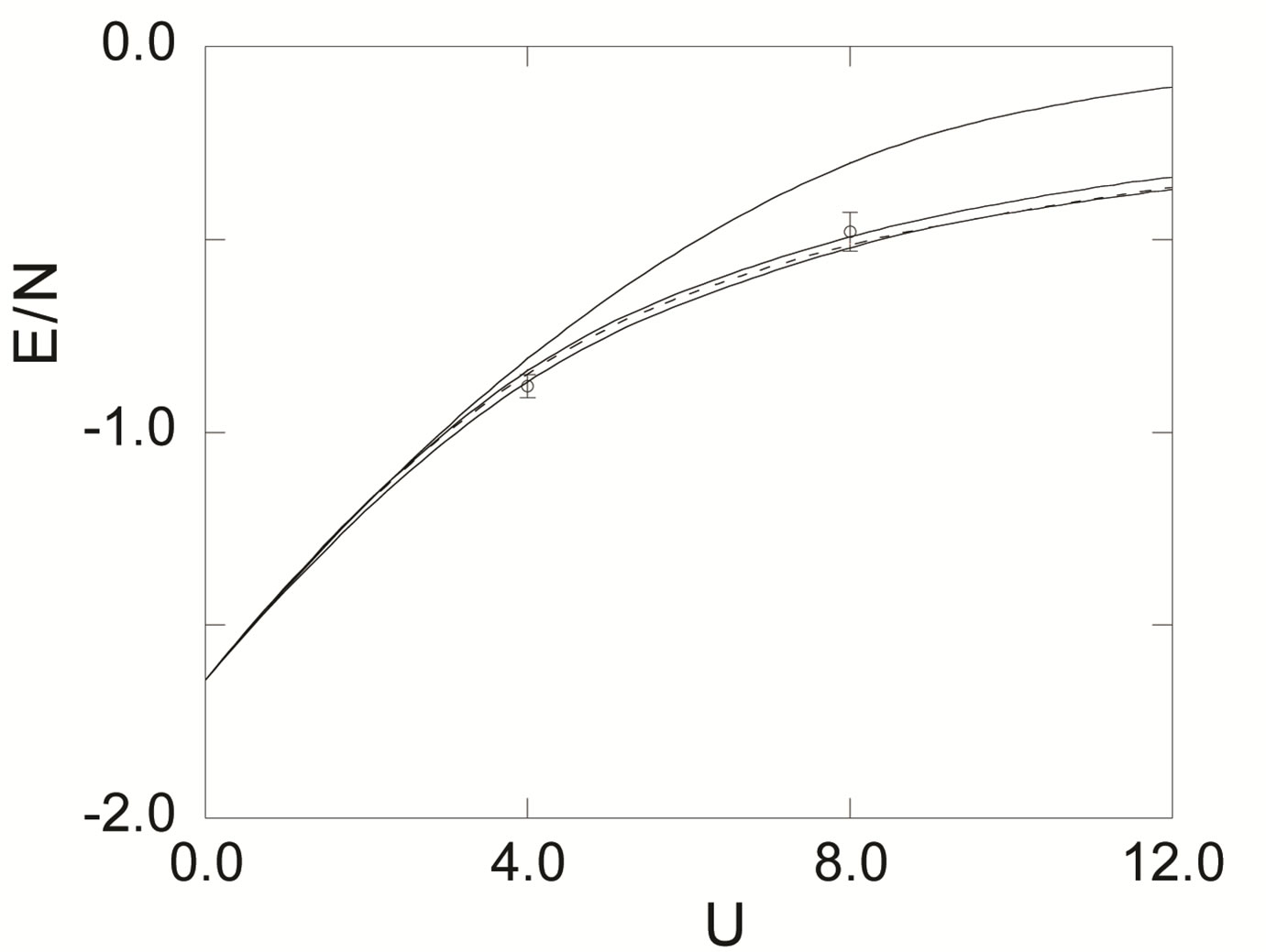
Figure 32. Energy as a function of  for 8 × 8 lattice at half-filling for the single-band Hubbard model. From the top the energies for
 ,
,  ,
,  and extrapolated values are shown. The quantum Monte Carlo results are shown by open circles [95].

Figure 33. The energy versus  for the single-band Hubbard model on the lattice of 10 × 10 sites. Solid and open symbols are obtained for
  with the normal and d-wave state initial functions
  and
and , respectively. Parameters are given by
 ,
,  and
and  [96].
[96].
correlation operators compared to that for the Gutzwiller function. The energy in the d-wave SC state is always lower than that in the normal state for each . The energy gain in the SC state remains the same order after the multiplication of correlation factors.
3.11.  and
and 
Relationships between  and structural features in cuprate high-temperature superconductors are very interesting. Torrance and Metzger found the first such relationship between
  and the Madelung potential difference
  [156]. Here
  is the potential difference between Cu and O sites in the CuO
 plane.
  was found to increase with decreasing
 . There is an interesting tendency of increasing
  with increasing relative ratio of hole density at oxygen site against that at copper site [117].
Here we show the results obtained by using the perturbation theory [62-66], There have been many similar works by making some kind of approximation such as random phase approximation (RPA) [157-159], fluctuation-exchange approximation (FLEX) [160-163], effective spin-fluctuation method [4,164,165], and perturbation theory in terms of U [166-168]. An application was made for Sr2RuO4 where we need to consider th emulti-band structure α and β orbitals [169], and also to the three-dimensional d-p model [170]. In our formulation the gap function is written as
 (62)
(62)
The exponent  indicates the strength of superconductivity. The results are in Figures 34 and 35 [171]. As shown in the figure, for positive
 , with increase of
  the exponent
  increases monotonously. This means the increase of superconducting gap and so of
 , and is consistent with the wide-range tendency of the variational Monte Carlo calculation [24,172]. This tendency can be understood in terms of
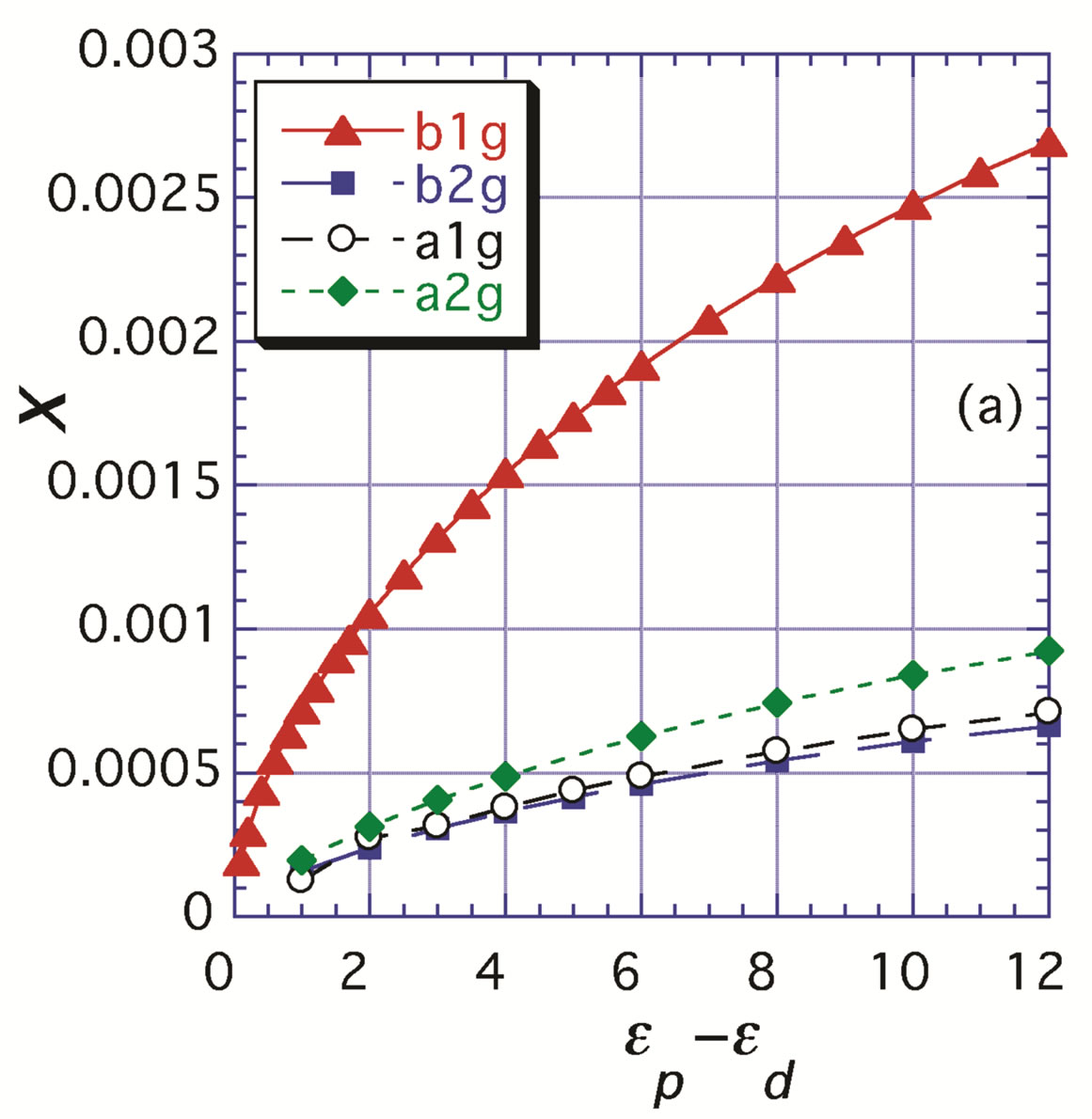
Figure 34. The exponent x (superconductivity strength) as a function of , where the level difference
  is positive.
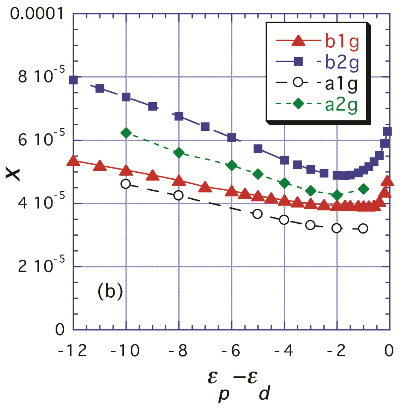
Figure 35. The exponent x as a function of , where the level difference
  is negative.
 (63)
(63)
where  is the weight ofd electrons. This clearly indicates that increase of
  leads to the increase of
  and subsequently of
 . In the case of
 , we take account of finite Coulomb repulsion
  on oxygen sites. The effective interaction coming from
  is similarly given by the susceptibility with the weight of
  electrons. The results of
  with
with  indicates that all four types of even parity (
 ,
,  ,
,  and
and ) SC strength values increase, so that
  is raised, as the absolute value
  increases in this region. This result shows that
  also plays an important role as well.
Let us give a discussion on this result. Increase of  in the region of
  means decrease of
  since
since
 , where
  is the second electron affinity of oxygen atom and
  is the third electron ionicity of copper atom and
  is the charge of electron. Therefore, this relation is consistent with the systematics reported in [156]. With increase of the distance of the apex oxygen away from the CuO2 plane, cuprate superconductors are known to increase
  [173]. The accompanying raise of
  should tend to increase
 .
.
The Coulomb interaction between p electrons on oxygen atom will raise the level of p electrons effectively. This leads to the lowering of p hole level  or the raise of
  relatively. This indicates that
  will be increased by the Coulomb interaction between p electrons.
4. Quantum Monte Carlo Studies
4.1. Quantum Monte Carlo Method
The Quantum Monte Carlo (QMC) method is a numerical method that is employed to simulate the behavior of correlated electron systems. We outline the QMC method in this section. The Hamiltonian is the Hubbard model that contains the on-site Coulomb repulsion and is written as
 (64)
(64)
where 
 is the creation (annihilation) operator of an electron with spin
  at the
  -th site and
 .
.  is the transfer energy between the sites
  and
and .
.  for the nearest-neighbor bonds. For all other cases
 .
.  is the on-site Coulomb energy. The number of sites is
  and the linear dimension of the system is denoted as
 . The energy unit is given by
  and the number of electrons is denoted as
 .
.
In a Quantum Monte Carlo simulation, the ground state wave function is
 (65)
(65)
where  is the initial one-particle state represented by a Slater determinant. For large
 ,
,  will project out the ground state from
 . We write the Hamiltonian as
  where K and V are the kinetic and interaction terms of the Hamiltonian in Equation (64), respectively. The wave function in Equation (65) is written as
 (66)
(66)
for . Using the Hubbard-Stratonovich transformation [27,94], we have
 (67)
(67)
for  or
or . The wave function is expressed as a summation of the one-particle Slater determinants over all the configurations of the auxiliary fields
 . The exponential operator is expressed as
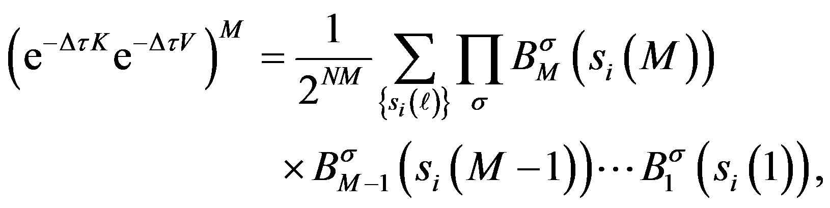 (68)
(68)
where we have defined
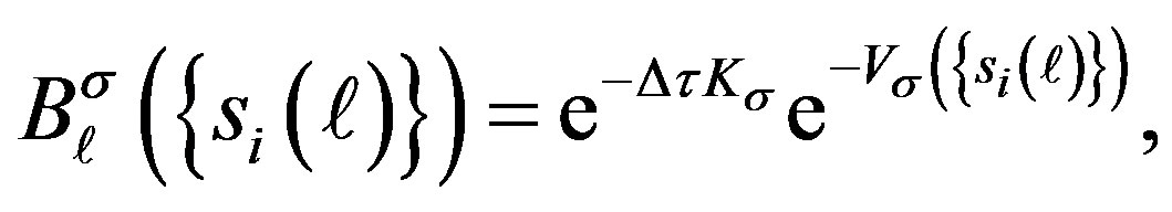 (69)
(69)
for
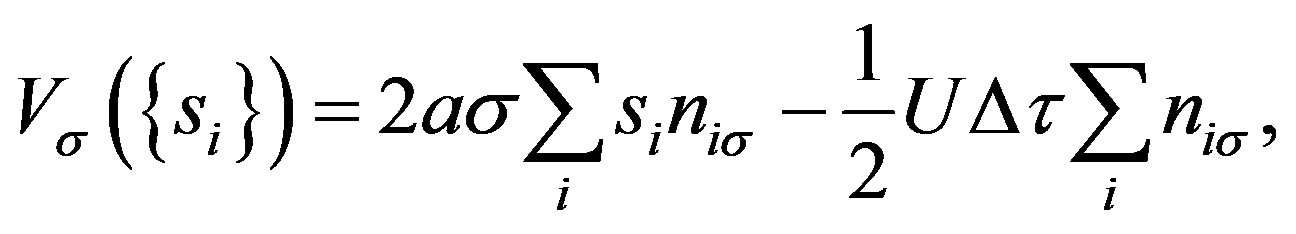 (70)
(70)
 (71)
(71)
The ground-state wave function is
 (72)
(72)
where  is a Slater determinant corresponding to a configuration
 of the auxiliary fields:
 (73)
(73)
The coefficients  are constant real numbers:
 . The initial state
  is a one-particle state. If electrons occupy the wave numbers
  for each spin
 ,
,  is given by the product
  where
where  is the matrix represented as [31]
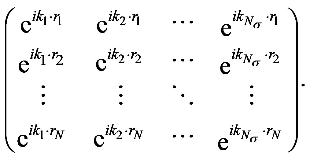 (74)
(74)
 is the number of electrons for spin
 . In actual calculations we can use a real representation where the matrix elements are
  or
or . In the real-space representation, the matrix of
  is a diagonal matrix given as
 (75)
(75)
The matrix elements of  are
are
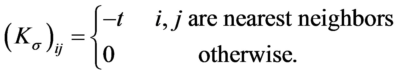 (76)
(76)
 is an
is an  matrix given by the product of the matrices
 ,
,  and
and . The inner product is thereby calculated as a determinant [38],
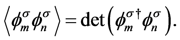 (77)
(77)
The expectation value of the quantity  is evaluated as
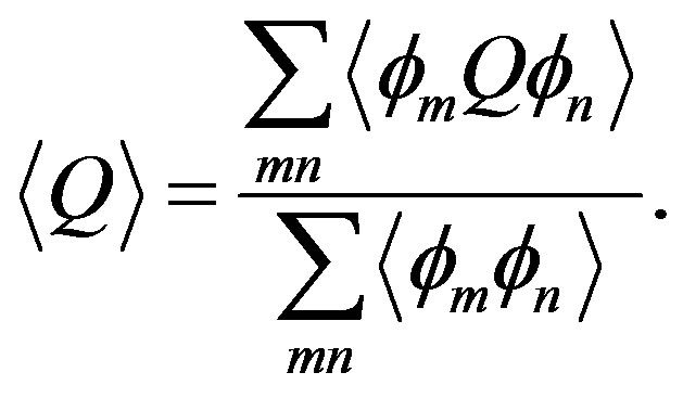 (78)
(78)
If  is a bilinear operator
  for spin
 , we have
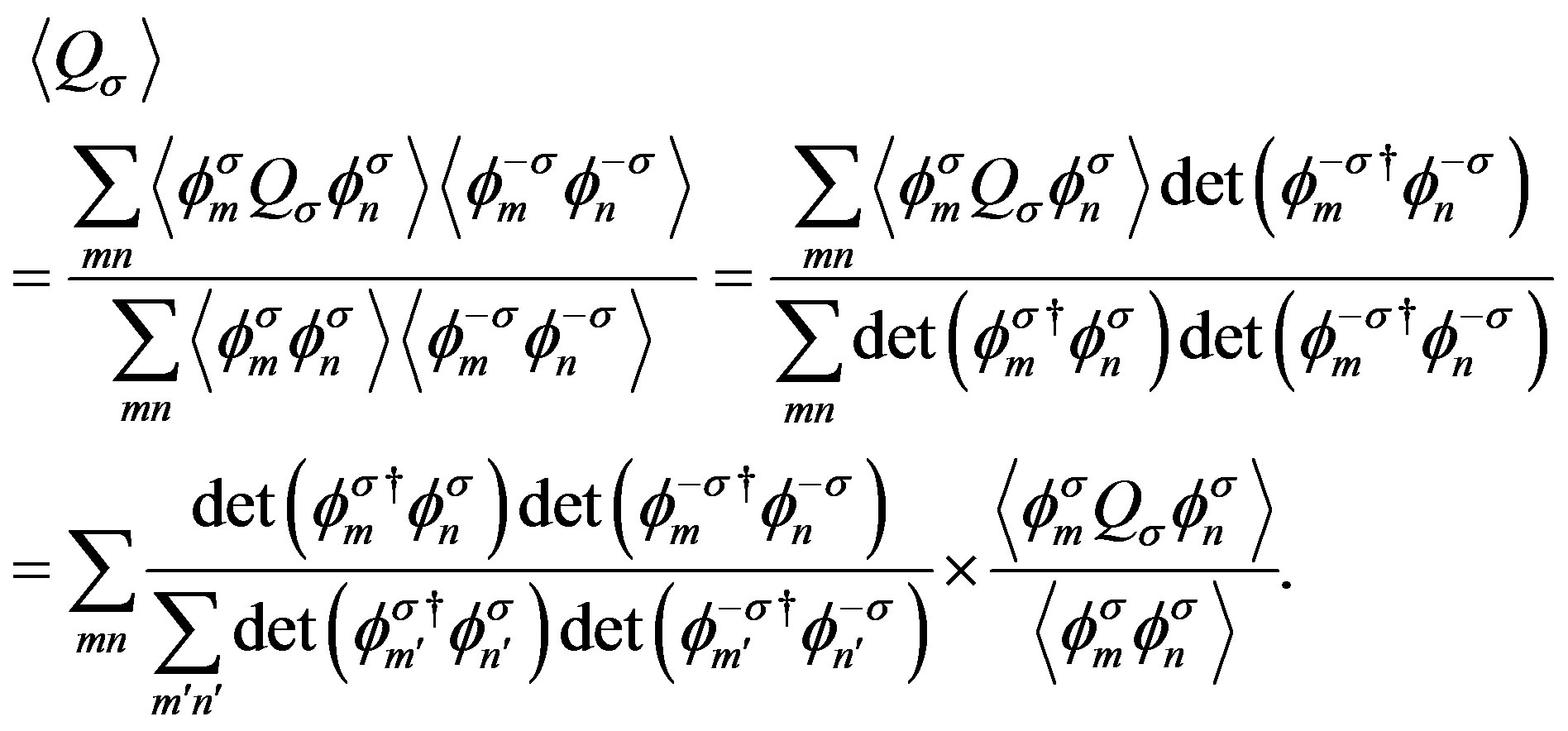 (79)
(79)
The expectation value with respect to the Slater determinants  is evaluated using the singleparticle Green’s function [31,38],
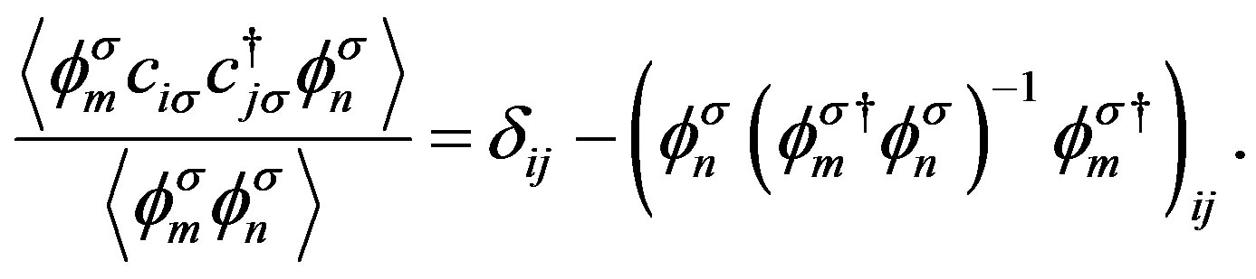 (80)
(80)
In the above expression,
 (81)
(81)
can be regarded as the weighting factor to obtain the Monte Carlo samples. Since this quantity is not necessarily positive definite, the weighting factor should be ; the resulting relationship is,
 (82)
(82)
where  and
and
 (83)
(83)
This relation can be evaluated using a Monte Carlo procedure if an appropriate algorithm, such as the Metropolis or heat bath method, is employed [94]. The summation can be evaluated using appropriately defined Monte Carlo samples,
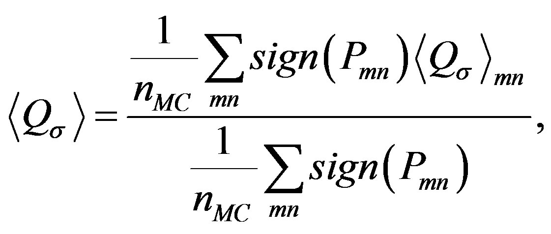 (84)
(84)
where  is the number of samples. The sign problem is an issue if the summation of
  vanishes within statistical errors. In this case it is indeed impossible to obtain definite expectation values.
4.2. Quantum Monte Carlo Diagonalization
4.2.1. Basic Method and Optimization
Quantum Monte Carlo diagonalization (QMD) is a method for the evaluation of  without the negative sign problem [41]. A bosonic version of this method was developed before in Ref.[174]. The configuration space of the probability
  in Equation (84) is generally very strongly peaked. The sign problem lies in the distribution of
  in the configuration space. It is important to note that the distribution of the basis functions
 is uniform since
  are constant numbers:
 . In the subspace
 , selected from all configurations of auxiliary fields, the right-hand side of Equation (78) can be determined. However, the large number of basis states required to obtain accurate expectation values is beyond the current storage capacity of computers. Thus we use the variational principle to obtain the expectation values.
From the variational principle,
 (85)
(85)
where 
 are variational parameters. In order to minimize the energy
 (86)
(86)
the equation 
 is solved for,
 (87)
(87)
If we set
 (88)
(88)
 (89)
(89)
the eigen-equation is
 (90)
(90)
for . Since
 are not necessarily orthogonal,
  is not a diagonal matrix. We diagonalize the Hamiltonian
 , and then calculate the expectation values of correlation functions with the ground state eigenvector.
In Quantum Monte Carlo simulations an extrapolation is performed to obtain the expectation values for the ground-state wave function. If  is large enough, the wave function in Equation (72) will approach the exact ground-state wave function,
  , as the number of basis functions,
  , is increased. If the number of basis functions is large enough, the wave function will approach,
  , as
, as  is increased. In either case the method employed for the reliable extrapolation of the wave function is a key issue in calculating the expectation values. The variance method was recently proposed in variational and Quantum Monte Carlo simulations, where the extrapolation is performed as a function of the energy variance. We can expect linearity in some cases [175]:
 (91)
(91)
where  denotes the variance defined as
 (92)
(92)
and  is the expected exact value of the quantity
 .
.
The simplest procedure for optimizing the groundstate wave function is to increase the number of basis states  by random sampling. First, we set
  and
and , for example,
  , and
, and . We denote the number of basis functions as
 . We start with
  and then increase up to 10,000. This procedure can be outlined as follows:
1) Generate the auxiliary fields 
 in
in  randomly for
  for
for 
 , and generate
  basis wave function
 .
.
2) Evaluate the matrices  and
and , and diagonalize the matrix
  to obtain
 . Then calculate the expectation values and the energy variance.
3) Repeat the procedure from 1) after increasing the number of basis functions.
For small systems this random method produces reliable energy results. The diagonalization plays an importance producing fast convergence. In order to lower the ground-state energy efficiently, we can employ a genetic algorithm [176] to generate the basis set from the initial basis set. One idea is to replace some parts of 
 in
in  that has the large weight
  to generate a new basis function
 . The new basis function
  obtained in this way is expected to also have a large weight and contribute to
 . The details of the method are shown in Ref.[41].
4.2.2. Ground State Energy and Correlation Functions
The energy as a function of the variance is presented in Figures 36-38 for ,
,  and
and , respectively. To obtain these results the genetic algorithm was employed to produce the basis functions except the open symbols in Figure 4. The
  where
where  in Figure 2 is the energy for the closed shell case up to 2000 basis states. The other two figures are for open shell cases, where evaluations were performed up to 3000 states. We show the results for the
 ,
,  and
and  systems in Table 2.
The Figure 39 is the momentum distribution function ,
,
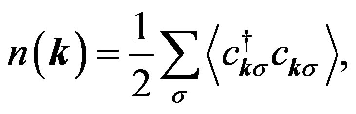 (93)
(93)
for  sites where the results for the Gutzwiller VMC and the QMD are indicated. The Gutzwiller function gives the results that
  increases as
  approaches
  from above the Fermi surface. This is clearly unphysical. This flaw of the Gutzwiller function near the Fermi surface is not observed for the QMD result.
4.2.3. Spin Gap in the Hubbard Ladder
Here we show the results for one-dimensional models. The ground state of the 1D Hubbard model is no longer Fermi liquid for . The ground state is insulating at half-filling and metallic for less than half-filling. The Figure 40 is the spin and charge correlation functions,
  and
and , as a function of the wave number, for

Table 2. Ground state energy per site from the Hubbard model. The boundary conditions are periodic in both directions. The current results are presented under the column labeled QMD. The constrained path Monte Carlo (CPMC) results are from Ref.[38]. The column VMC is the results obtained for the optimized variational wave function  except for 6 × 2 for which
  is employed. The QMC results are from Ref.[35]. Exact results are obtained using diagonalization [177].
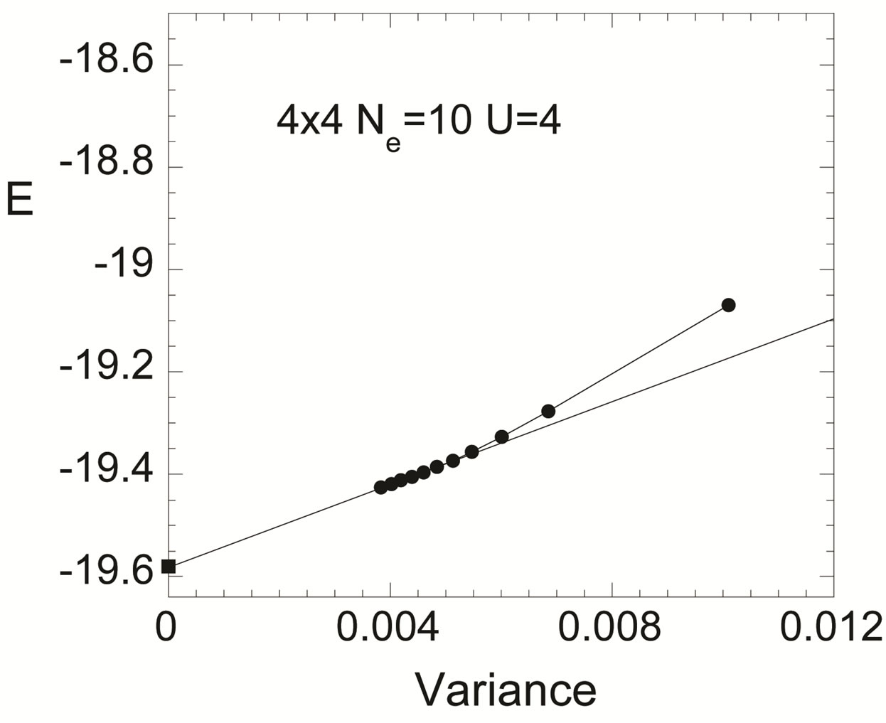
Figure 36. Energy as a function of the variance for 4 × 4,  and
and . The square is the exact result. The data fit using a straight line using the least-square method as the variance is reduced. We started with
  (first solid circle) and then increase up to 2000.
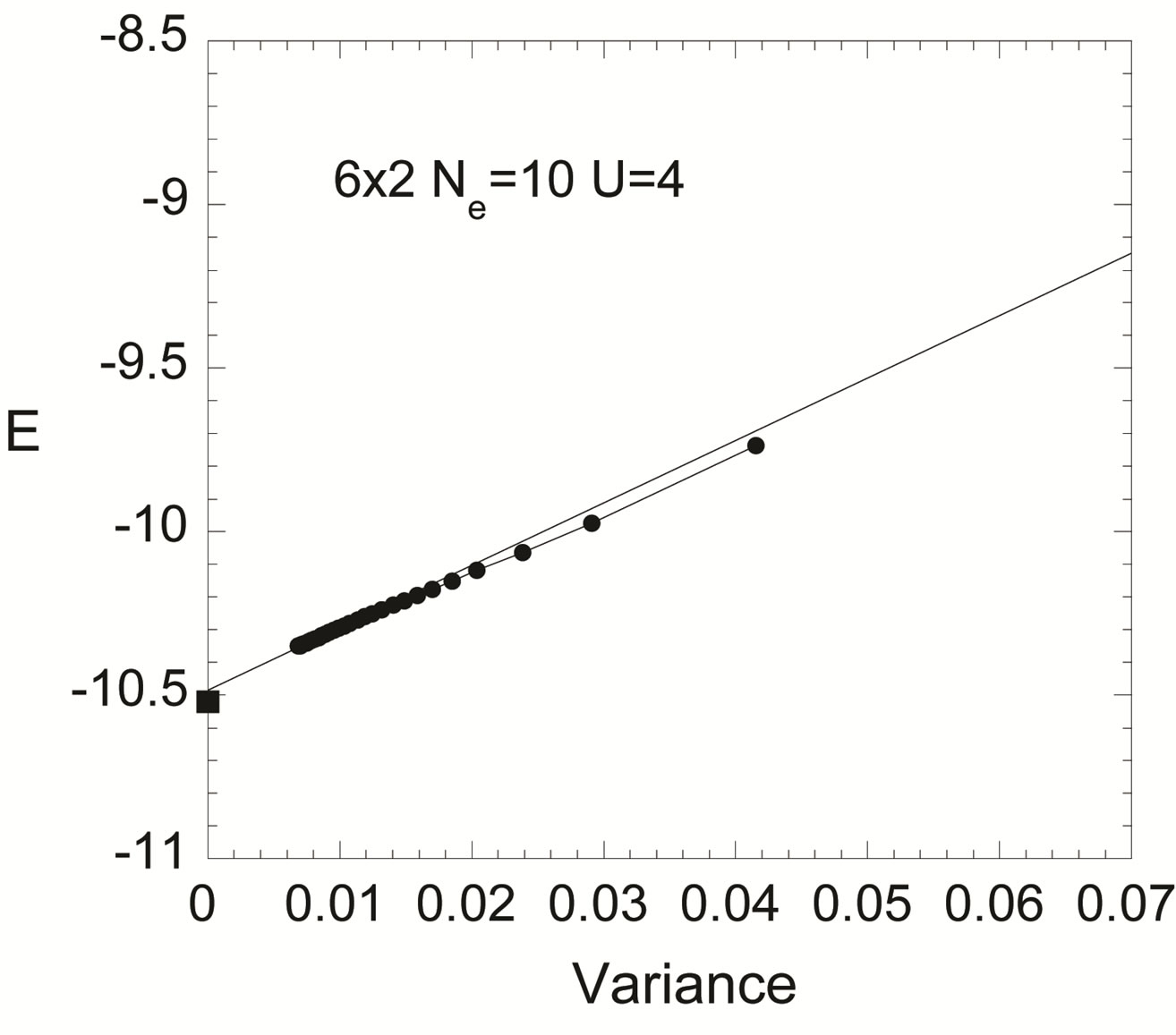
Figure 37. Energy as a function of the variance for 6 × 2  and
and . The square is the exact value obtained using exact diagonalization.

Figure 38. Energy as a function of the variance  for 6 × 6. with the periodic boundary conditions. Solid circles and crosses are data obtained from the QMD method for two different initial configurations of the auxiliary fields. Gray open circles show results obtained from the
  -renormalization method with 300 basis wave functions.
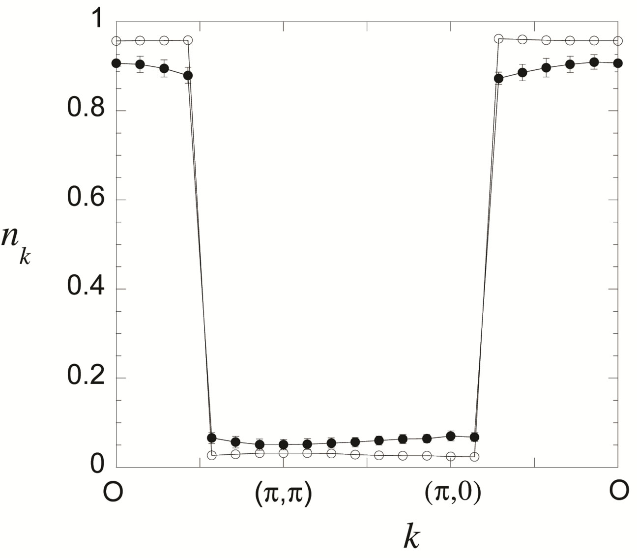
Figure 39. Momentum distribution function for the 14 × 14 lattice. Parameters are  and
and . The boundary conditions are periodic in both directions. The results for the Gutzwiller function (open circle) are also provided.
the 1D Hubbard model where . The
. The  singularity can be clearly identified where the dotted line is for
 . The spin correlation is enhanced and the charge correlation function is suppressed slightly because of the Coulomb interaction.
The spin correlation function  for the Hubbard ladder is presented in Figure 41, where
  and
and .
.  is defined as
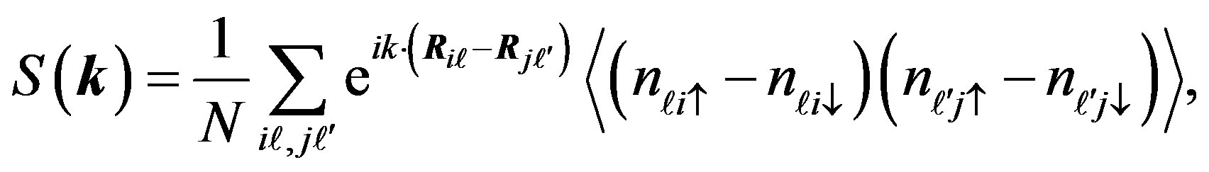 (94)
(94)
where  denotes the site
 . We use the convention that
  where
where  and
and  indicate the lower band and upper band, respectively. There are four singularities at
 ,
,  ,
,  , and
, and  for the Hubbard ladder, where
  and
and  are the Fermi wave numbers of the lower and upper band, respectively.
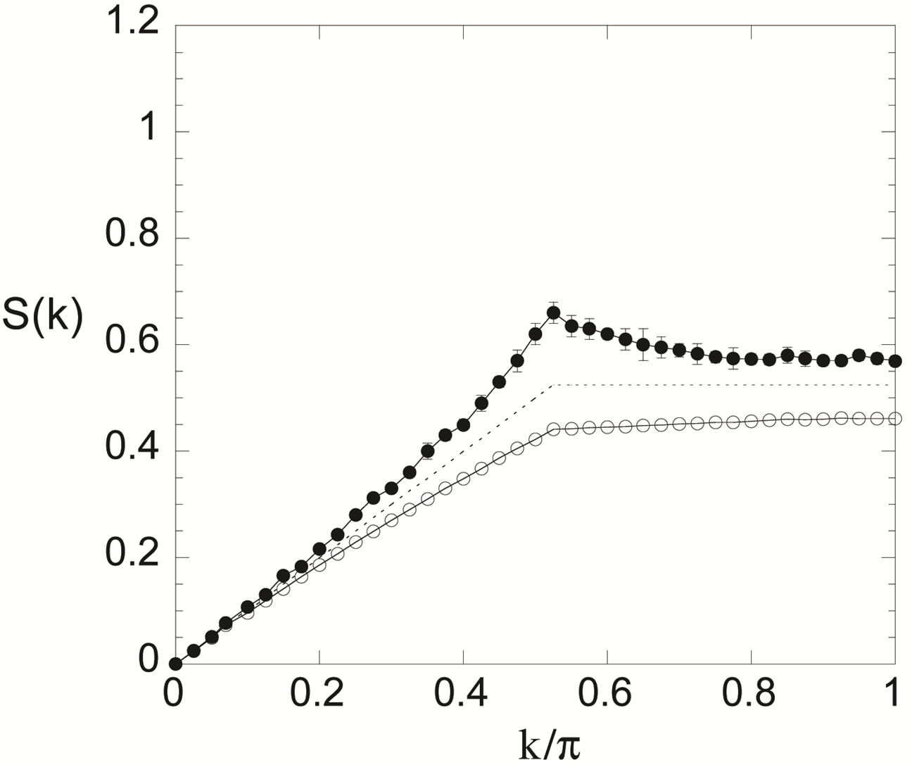
Figure 40. Spin (solid circle) and charge (open circle) correlation functions obtained from the QMD method for the one-dimensional Hubbard model with 80 sites. The number of electrons is 66. We set  and use the periodic boundary condition.
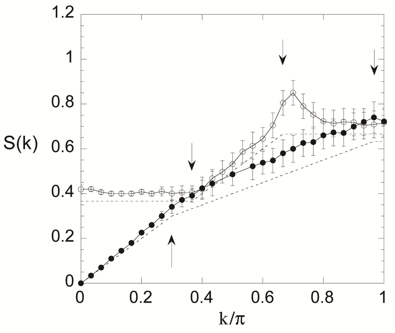
Figure 41. Spin correlation function obtained from the QMD method for the ladder Hubbard model for 60 × 2 sites with periodic boundary condition. The number of electrons is 80 and . The upper line is for the upper band and the lower line is for the lower band. Singularities are at
 ,
,  ,
,  and
and  from left. The dotted lines are for
 .
.
It has been expected that the charge gap opens up as  turns on at half-filling for the Hubbard ladder model. In Figure 42 the charge gap at half-filling is shown as a function of
 . The charge gap is defined as
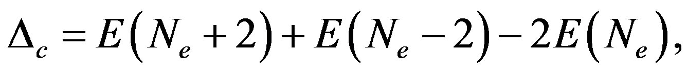 (95)
(95)
where  is the ground state energy for the
  electrons. The charge gap in Figure 42 was estimated using the extrapolation to the infinite system from the data for the
 ,
,  , and
, and  systems. The data suggest the exponentially small charge gap for small
  or the existence of the critical value
  in the range of
 , below which the charge gap vanishes.
4.2.4. Magnetization in 2D Hubbard Model
The ground state of the 2D Hubbard model at half-filling is antiferromagnetic for  because of the nesting due to the commensurate vector
 . The Gutzwiller function predicts that the magnetization
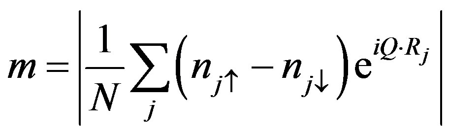 (96)
(96)
increases rapidly as  increases and approaches
  for large
 . In Figure 43, the QMD results are presented for
  as a function of
 . The previous results obtained using the QMC method are plotted as open circles. The gray circles are for the
  -function VMC method and squares are the Gutzwiller VMC data. Clearly, the magnetization is reduced considerably because of the fluctuations, and is smaller than the Gutzwiller VMC method by about 50 percent.
4.3. Pair Correlation Function
The pair correlation function  is defined by
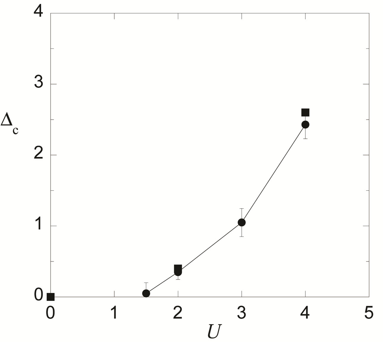
Figure 42. Charge gap as a function of  for
for  (circles). The DMRG results (squares) are provided for comparison [58].
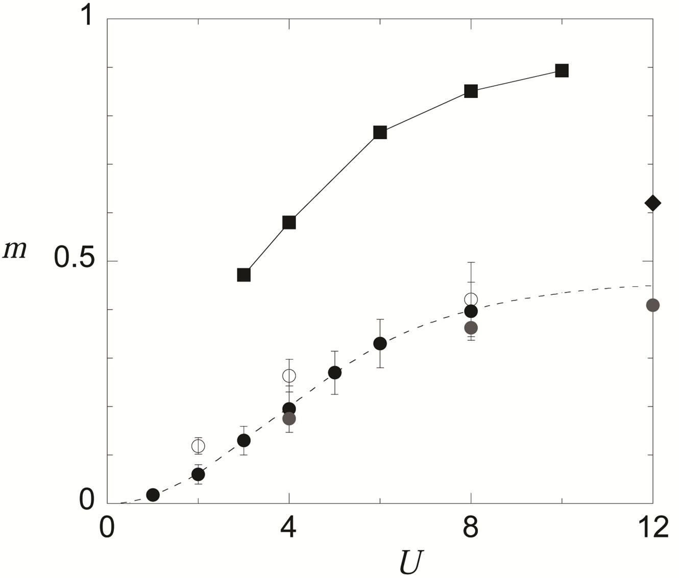
Figure 43. Magnetization as a function of  for the halffilled Hubbard model after extrapolation at the limit of large N. Solid circles are the QMD results, and open circles are results obtained from the QMC method [28]. The squares are the Gutzwiller-VMC results [43] and gray solid circles show the 3rd
  -function
  VMC results carried out on the 8 × 8 lattice [95]. The diamond symbol is the value from the two-dimensional Heisenberg model where
  [179,180].
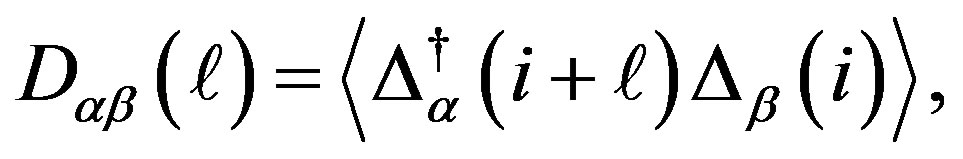 (97)
(97)
where  ,
,  , denote the annihilation operators of the singlet electron pairs for the nearestneighbor sites:
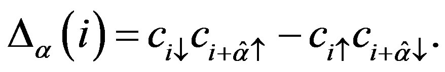 (98)
(98)
Here  is a unit vector in the
  -direction. We consider the correlation function of d-wave pairing:
 (99)
(99)
where
 (100)
(100)
 and
and  denote sites on the lattice.
We show how the pair correlation function is evaluated in quantum Monte Carlo methods. We show the pair correlation functions  and
and  on the lattice
  in Figures 44 and 45. The boundary condition is open in the 4-site direction and is periodic in the other direction. An extrapolation is performed as a function of
  in the QMC method with Metropolis algorithm and as a function of the energy variance
  in the QMD method with diagonalization. We keep
  a small constant
  and and increase
 , where
  is the division number. In the Metropolis QMC method, we calculated averages over
  Monte Carlo steps. The exact values were obtained by using the exact diagonalization method. Two methods give consistent results as shown in figures. All

Figure 44. Pair correlation function  and
and  for 4 × 3,
  and
and  obtained by the diagonalization quantum Monte Carlo method. The square are the exact results obtained by the exact diagonalization method. The data fit using a straight line using the least-square method as the variance is reduced. We started with
  (first solid circles) and then increase up to 2000.

Figure 45. Pair correlation function  and
and  for 4 × 3,
  and
and  obtained by the Metropolis quantum Monte Carlo method. The square are the exact results obtained by the exact diagonalization method. An extrapolation is performed as a function of
 .
.
the  and
and  are suppressed on
  as
as  is increased. In general, the pair correlation functions are suppressed in small systems. In Figures 46 and 47, we show the inter-chain pair correlation function for the ladder model
 . We use the open boundary condition. The number of electrons is
 , and the strength of the Coulomb interaction is
 .
.  indicates the electron pair along the rung, and
  is the expectation value of the parallel movement of the pair along the ladder. The results obtained by two methods are in good agreement except
  (nearest-neighbor correlation).
We first consider the half-filled case with ; in this case the antiferromagnetic correlation is dominant over the superconductive pairing correlation and thus the pairing correlation function is suppressed as the Coulomb repulsion
  is increased. The Figure 48 exhibits the d-wave pairing correlation function
  on
on  lattice as a function of the distance. The
  is suppressed due to the on-site Coulomb interaction, as expected. Its reduction is, however, not so considerably large compared to previous QMC studies [39] where the pairing correlation is almost annihilated for
 . We then turn to the case of less than half-filling. We show the results on
  with electron number
 . We show
  as a function of the distance in Figure 49
 . In the scale of this figure,
  for
for  is almost the same as that of the non-interacting case, and is enhanced slightly for large
 . Our results indicate that the pairing correlation is not suppressed and is indeed enhanced by the Coulomb interaction
 , and its enhancement is very small.
The Figure 50 shows  on
on  lattice. This also indicates that the pairing correlation function is
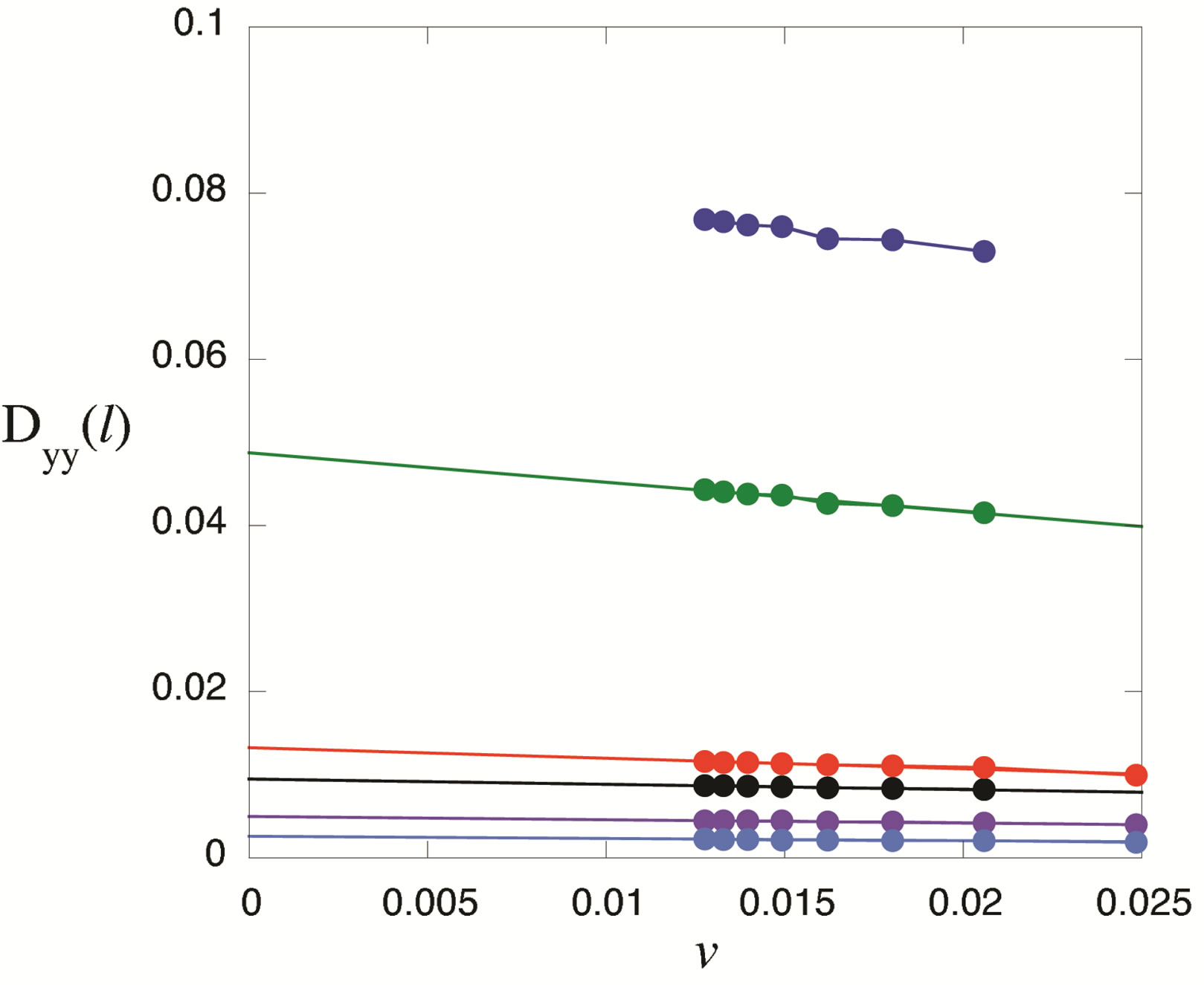
Figure 46. Pair correlation function  as a function of the energy variance
  for 30 × 2,
  and
and  obtained by the diagonalization quantum Monte Carlo method.
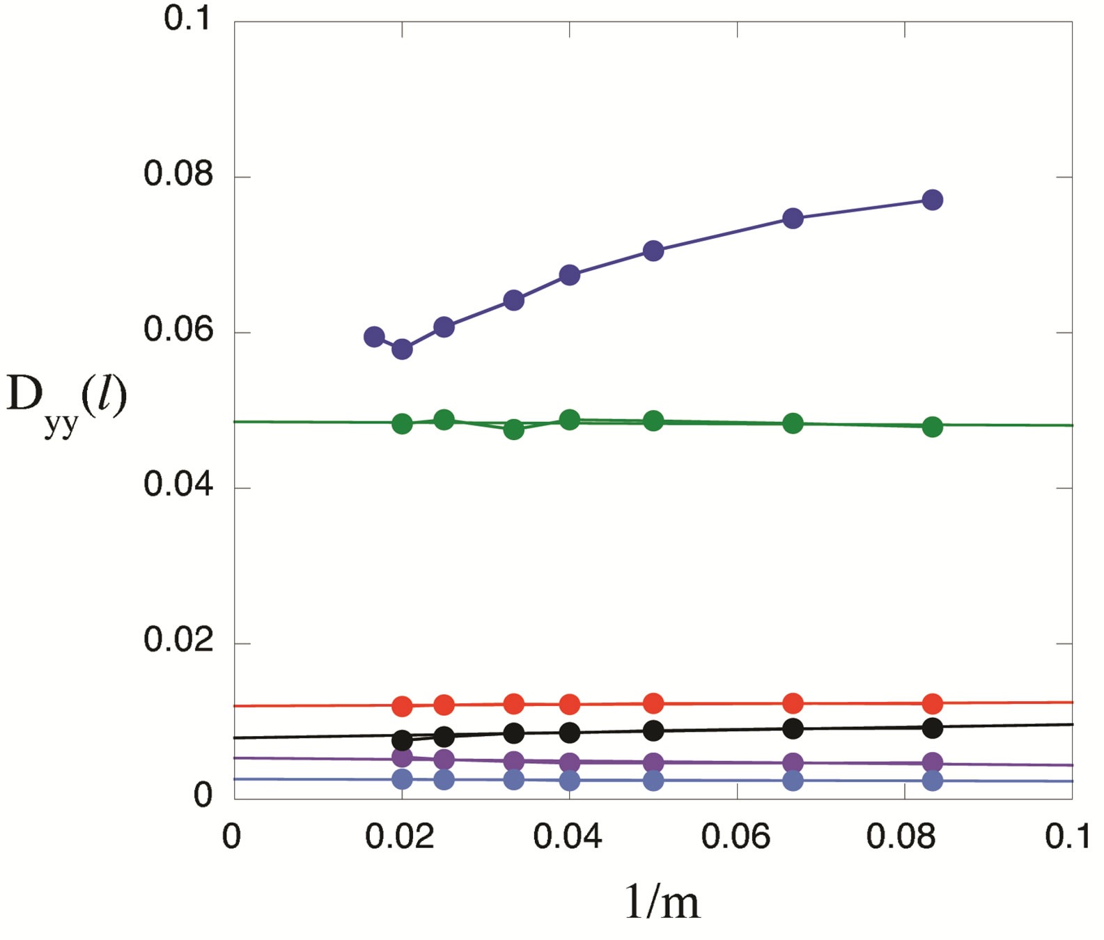
Figure 47. Pair correlation function  as a function of
  for 30 × 2,
  and
and  obtained by the Metropolis quantum Monte Carlo method.
enhanced for . There is a tendency that
  is easily suppressed as the system size becomes small. We estimated the enhancement ratio compared to the non-interacting case
 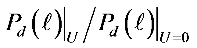 at
at 
for  as shown in Figure 51. This ratio increases as the system size is increased. To compute the enhancement, we picked the sites, for example on
  lattice,
  , (4,0), (4,1), (3,3), (4,2), (4,3), (5,0), (5,1) with
  and evaluate the mean value. In our computations, the ratio increases almost linearly indicating a possibility of superconductivity. This indicates
  for
for .
.
Because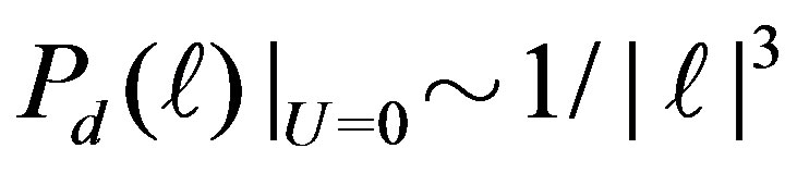 , we obtain
 for
for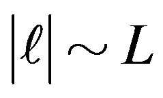 . This indicates that the exponent of the power law is 2. When
 , the
, the
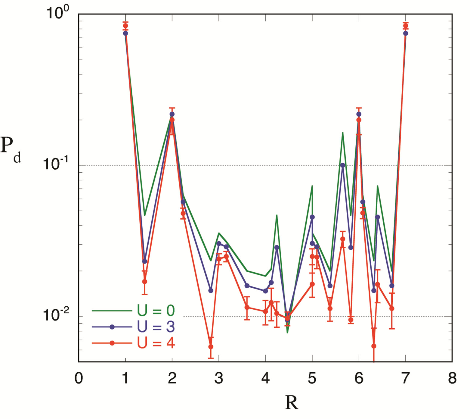
Figure 48. Pair correlation function  as a function of the distance
  on 8 × 8 lattice for the half-filled case
 . We set
  and
and , 3 and 4. To lift the degeneracy of electron configurations at the Fermi energy in the half-filled case, we included a small staggered magnetization
  in the initial wave function
 .
.

Figure 49. Pair correlation function  as a function of the distance
  on 8 × 8 lattice for
 . We set
  and
and , 4 and 6.
enhancement is small and is almost independent of . In the low density case, the enhancement is also suppressed being equal to 1. In Figure 52, the enhancement ratio is shown as a function of the electron density
  for
for . A dome structure emerges even in small systems. The square in Figure 52 indicates the result for the half-filled case with
  on
on  lattice. This is the open shell case and causes a difficulty in computations as a result of the degeneracy due to partially occupied electrons. The inclusion of
  enhances
  compared to the case with
  on
on  lattice.
  is, however, not enhanced over the non-interacting case at half-filling. This also holds for
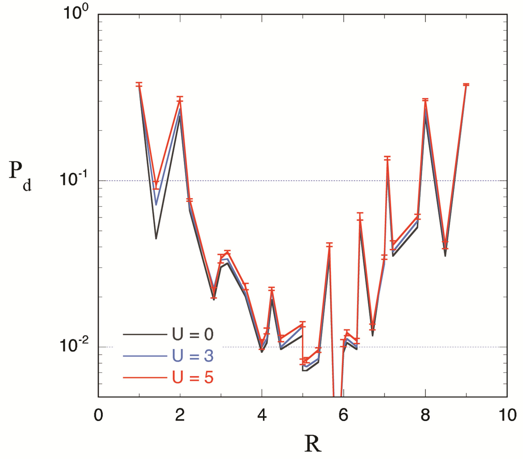
Figure 50. Pair correlation function  as a function of the distance
  on 10 × 10 lattice for
  and
and  . The strength of the Coulomb interaction is
 , 3 and 5.

Figure 51. Enhancement ratio of pair correlation function  as a function of the linear system size L for
  and
and . The electron density
  is about 0.8:
  for squares. The data for
  and
and  are also shown by circles.
 lattice where the enhancement ratio
 . This indicates the absence of superconductivity at half-filling.
4.4. Spin Susceptibility
We propose a method to compute the magnetic susceptibility at absolute zero  [178]. We add the source term
  to the Hamiltonian as follows
 (101)
(101)
where  is a small real number of the order
  or
or . We calculate
  in the ground state, which is, as shown by the linear response theory, the magnetic susceptibility
 (102)
(102)
in the limit of small , where
  is the retarded Green function and
  is the dynamical susceptibility,
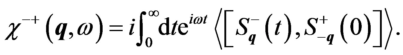 (103)
(103)
Indeed, the above formula gives the correct spin susceptibility  on the finite lattice for the noninteracting case, which is given by
  with the Fermi distribution function
 . We calculate
  by using the quantum Monte Carlo method to obtain
 .
.
We examine the results obtained for the susceptibilities. Figure 53 shows the spin susceptibility  for
for  on a
on a  lattice as a function of
  or the energy variance
 . The number of electrons is 10. The expectation values agree well with exact values given by the exact diagonalization method.
We now compute the staggered susceptibility  by adding the source term
 to the Hamiltonianwhere
 . Here we set the periodic and antiperiodic boundary conditions in the
  and
and  directions, respectively, to avoid a numerical difficulty caused by the degeneracy between states
  and
and 
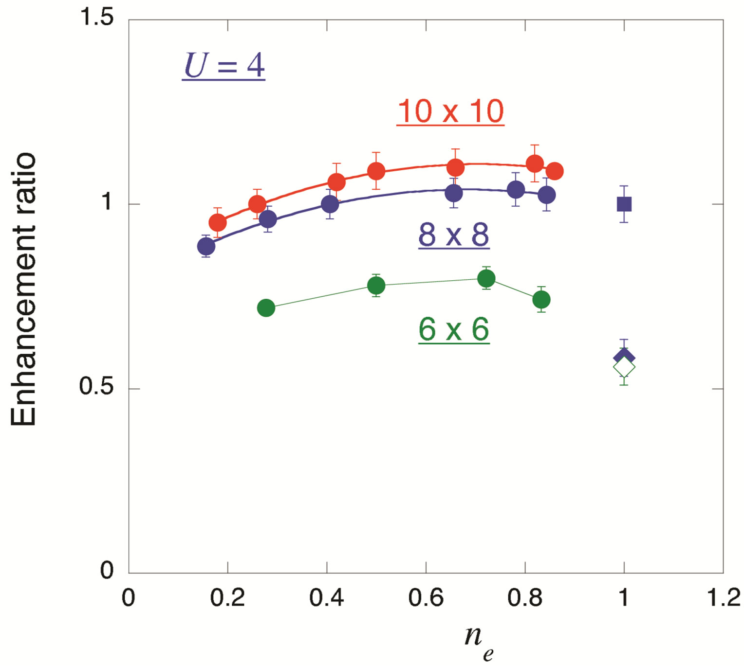
Figure 52. Enhancement ratio of pair correlation function  as a function of the electron density
 . We adopt
  and
and . For the half-filled case, the diamonds show that for
  on 8 × 8 lattice (solid diamond) and 6 × 6 lattice (open diamond). The square is for
  on 8 × 8 and 10 × 10 where there is no enhancement.
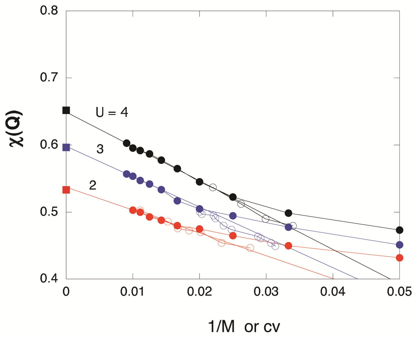
Figure 53. Spin susceptibility  as a function of
  or the variance
  for a 6 × 2 lattice with the periodic boundary condition. The number of electrons is 10. We set
 . The solid circles and open circles are obtained by using the QMC method and the QMD method, respectively. The squares indicate exact values. The variance
  is multiplied by a numerical constant. We set
 , 3, and 4 in units of t.
where . It has been shown that a long-range spin correlation exists in the ground state of the half-filled Hubbard model with
  for
for  [40, 41,179,180]. In the case
 ,
,  exhibits a double logarithmic behavior
 .
.  is shown as a function of
  in Figure 54 for
 , 3, and 4. The obtained values are well fitted by
  and
and  diverges in the limit of a large system size
 :
:
 (104)
(104)
This result is consistent with the existence of the long-range spin correlation for  [179,180]. The degree of divergence of
  is beyond the criterion of the Kosterlitz-Thouless transition, and thus the long-range order represented by
  belongs to a different category. The
  behavior of
  is consistent with the predictions of perturbation theory in the 2D non-linear sigma model at low temperatures [181].
4.5. Pair Susceptibility
In this section we consider a method to evaluate the pair susceptibility  at
at . In order to compute the pair susceptibility, we use an electron-hole transformation for the down spin,
  , whereas the up-spin electrons are unaltered,
 . For the on-site s-wave pairing, the source term is given by the following expression
 (105)
(105)
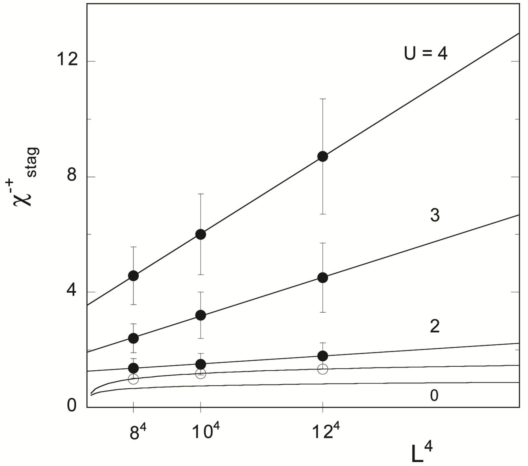
Figure 54. Staggered spin susceptibility  as a function of
  at half-filling with
  for
for , 3, and 4. We use the periodic and antiperiodic boundary conditions in the x and y directions, respectively. The lowest line is for
 , which is fitted by a logarithmic curve. The open circles show the results for the Gutzwiller function with
 , which exhibits a logarithmic dependence.
For the anisotropic d-wave pairing, we add
 (106)
(106)
where  and
and . The s-wave and d-wave pair susceptibility are respectively:
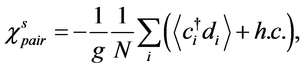
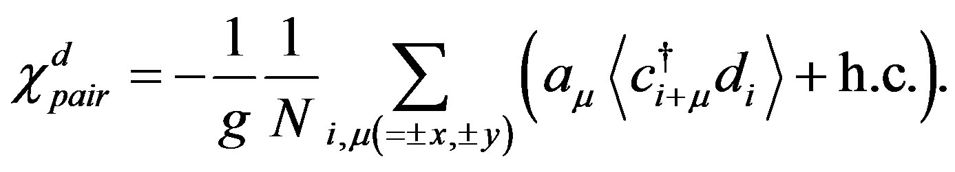 (107)
(107)
Using the Fourier transformation, the source term for the pair potential is written as follows 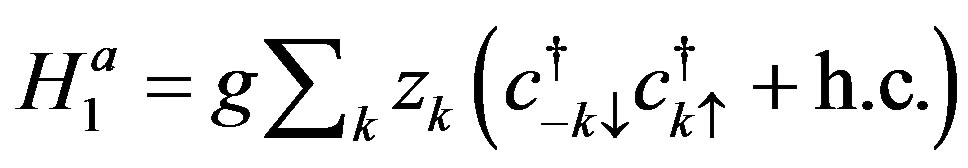 for
for  or
or  with the
  -dependence factor
 . If we define
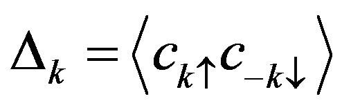 , then for a small value of
 , we have the following
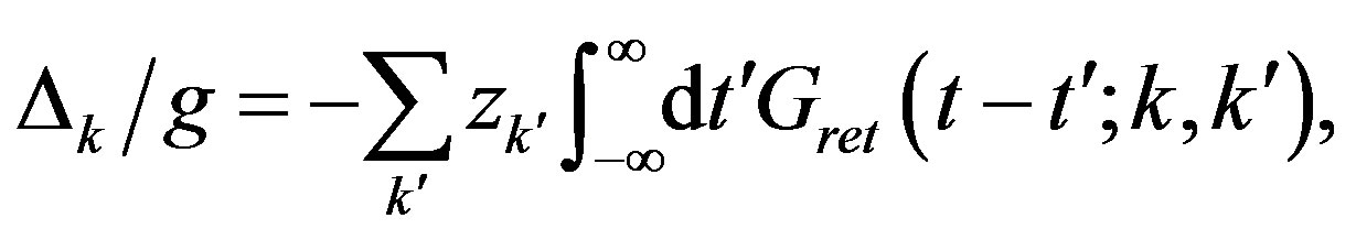 (108)
(108)
where
 (109)
(109)
for  and
and . On the basis of analytic continuation, using the thermal Green function,
  is written as
 (110)
(110)
In the noninteracting system, this formula exhibits logarithmic divergence on the finite lattice :
:  with constants
  and
and , which can be confirmed by numerical estimations on finite systems.
In the Kosterlitz-Thouless theory, the susceptibility is scaled as follows [182,183]: , where
  is the coherence length.
  is of order
  on a lattice
  if long-range coherence exists. The exponent
  is expected to be 0 at absolute zero. Thus
  scales as
  in the ground state if the Kosterlitz-Thouless transition occurs at some temperature.
First, we investigate  for the attractive Coulomb interaction
 . For this model, the existence of a Kosterlitz-Thouless transition has been predicted on the basis of quantum Monte Carlo methods [34,183]. The results in Figure 55 show that the size dependence for
  and
and  is
is
 (111)
(111)
which is consistent with previous studies, and shows the existence of a Kosterlitz-Thouless transition for the attractive interaction. At near half-filling,  is more enhanced than that at
 . Second, let us investigate the d-wave pair susceptibility
  for the repulsive Coulomb interaction. Pair susceptibilities are
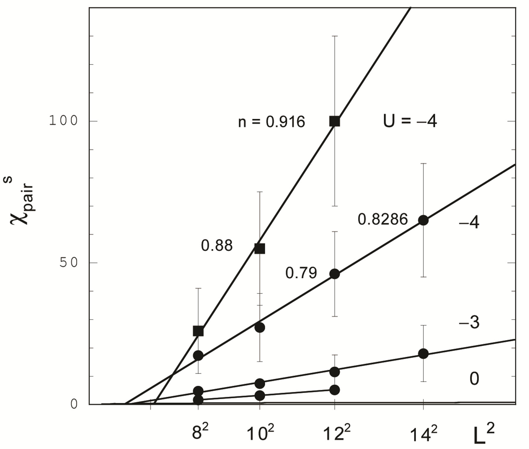
Figure 55. Isotropic  -wave susceptibility
  as a function of
  for the negative-U Hubbard model with
 , -3, and -4, and
 . The circles indicate the results for
 , where we use the periodic boundary condition in both the x and y directions, and the chemical potential is set at the center of the level spacing between adjacent energy levels. The lowest dotted line is for
 , which is fitted by a logarithmic curve, that is,
 . We show
  for
for  and
and  by squares, where the boundary condition is antiperiodic in one direction and periodic in the other direction.
sensitively dependent on the band structure, particularly the energy of the van Hove singularity, as a characteristic of two-dimensional systems. We compute  at an electron density
 , a value near that of optimally doped high-temperature cuprates. We set
 . Figure 56 shows
  as a function of
  for
for , 3, 4, and 5 with
  and
and . This shows that
 (112)
(112)
if  is moderately large. This result shows that a d-wave superconducting Kosterlitz-Thouless transition may exist for the repulsive interaction if we adjust the band parameters in the region of optimal doping.
5. Summary
We have investigated the superconductivity of electronic origin on the basis of the (single-band and three-band) two-dimensional Hubbard model. First, we employ the variational Monte Carlo method to clarify the phase diagram of the ground state of the Hubbard model. The superconducting condensation energy per site obtained by the Gutzwiller ansatz is reasonably close to experimental value . We have examined the stability of striped and checkerboard states in the under-doped region. The relation of the incommensurability and hole density,
  , is satisfied in the
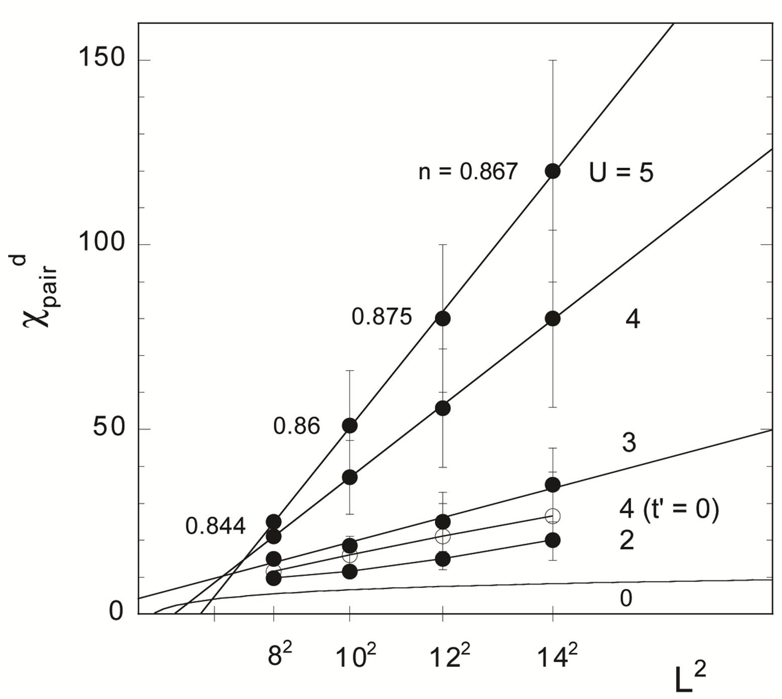
Figure 56. The d-wave susceptibility  as a function of
  for the repulsive-U Hubbard model with
 , 3, 4, and 5. We use the periodic boundary condition in both the x and y directions. The solid circles present the results with
  and
and  for
for , 3, 4 and 5. For the solid squares the parameters are
  and
and  with
with . The open squares are for
 ,
,  (near half-filling) and
 . The open circles indicate the results for
 ,
,  and
and . The lowest line for
  is fitted by a logarithmic curve:
 .
.
lower doped region. We have found that the  period checkerboard spin modulation is stabilized in the two-dimensional Hubbard model with the Bi-2212 type band structure.
We have further performed investigation by using the quantum Monte Carlo method that is an exact unbiased method. We have presented an algorithm of the quantum Monte Carlo diagonalization to avoid the negative sign problem in quantum simulations of many-fermion systems. We have computed d-wave pair correlation functions. In the half-filled case  is suppressed for the repulsive
 , and when doped away from half-filling
 ,
,  is enhanced slightly for
 . It is noteworthy that the correlation function
  is indeed enhanced and is increased as the system size increases in the 2D Hubbard model. The enhancement ratio increases almost linearly
  as the system size is increased, which is an indication of the existence of superconductivity. Our criterion is that when the enhancement ratio as a function of the system size
  is proportional to a certain power of
 , superconductivity will be developed. This ratio depends on
  and is reduced as
  is decreased. The dependence on the band filling shows a dome structure as a function of the electron density. In the
  system, the ratio is greater than 1 in the range
 . Let us also mention on superconductivity at half-filling. Our results indicates the absence of superconductivity in the half-filling case because there is no enhancement of pair correlation functions
6. Acknowledgements
We thank I. Hase, S. Koikegami, S. Koike and J. Kondo for stimulating discussions. This work was supported by a Grant-in Aid for Scientific Research from the Ministry of Education, Culture, Sports, Science and Technology of Japan, and CREST Program of Japan Science and Technology Agency. A part of numerical calculations was performed at the facilities in the Supercomputer Center of the Institute for Solid State Physics of the University of Tokyo.
REFERENCES
- J. G. Bednorz and K. A. Müller, Zeitschrift für Physik B Condensed Matter, Vol. 64, 1986, pp. 189-193. doi:10.1007/BF01303701
- E. Dagotto, Reviews of Modern Physics, Vol. 66, 1994, pp. 763-840.
- P. W. Anderson, “The Theory of Superconductivity in the High-Tc Cuprates,” Princeton University Press, Princeton, 1997.
- T. Moriya and K. Ueda, Advances in Physics, Vol. 49, 2000, pp. 555-606. doi:10.1080/000187300412248
- K. H. Bennemann and J. B. Ketterson, “The Physics of Superconductor,” Springer, Berlin, 2003.
- G. R. Stewart, Reviews of Modern Physics, Vol. 56, 1984, pp. 755-787.
- P. A. Lee, T. M. Rice, J. W. Serene, L. J. Sham and J. W. Wilkins, Comments on Condensed Matter Physics, Vol. 12, 1986, p. 99.
- H. R. Ott, Progress in Low Temperature Physics, Vol. 11, 1987, pp. 215-289. doi:10.1016/S0079-6417(08)60034-7
- M. B. Maple, “Handbook on the Physics and Chemistry of Rare Earths Vol. 30,” Elsevier, Amsterdam, 2000.
- T. Ishiguro, K. Yamaji and G. Saito, “Organic Superconductors,” Springer-Verlag, Berlin, 1998. doi:10.1007/978-3-642-58262-2
- C. C. Tsuei, et al., Physical Review Letters, Vol. 73, 1994, pp. 593-596.
- D. A. Wollman, et al., Physical Review Letters, Vol. 74, 1995, pp. 797-800.
- C. C. Tsuei and J. R. Kirtlry, Physical Review Letters, Vol. 85, 2000, pp. 182-185.
- T. Sato, T. Kamiyama, T. Takahashi, K. Kurahashi and K. Yamada, Science, Vol. 291, 2001, pp. 1517-1519. doi:10.1126/science.1058021
- T. Yanagisawa, S. Koikegami, H. Shibata, S. Kimura, S. Kashiwaya, A. Sawa, N. Matsubara and K. Takita, Journal of the Physical Society of Japan, Vol. 70, 2001, pp. 2833-2835. doi:10.1143/JPSJ.70.2833
- G. Shirane, Y. Endoh, R. Birgeneau, M. A. Kastner, Y. Hidaka, M. Oka, M. Suzuki and T. Murakami, Physical Review Letters, Vol. 59, 1987, p. 1613.
- K. B. Lyons, P. A. Fleury, L. F. Schncemmeyer and J. V. Waszczak, Physical Review Letters, Vol. 60, 1988, pp. 732-735.
- E. Manousakis and R. Salvadoe, Physical Review Letters, Vol. 62, 1989, pp. 1310-1313.
- P. Prelovsek, Physics Letters A, Vol. 126, 1988, pp. 287- 290. doi:10.1016/0375-9601(88)90764-5
- M. Inui and S. Doniach, Physical Review B, Vol. 38, 1988, pp. 6631-6635.
- T. Yanagisawa, Physical Review Letters, Vol. 68, 1992, pp. 1026-1029.
- T. Yanagisawa and Y. Shimoi, Physical Review B, Vol. 48, 1993, pp. 6104-6110.
- T. Yanagisawa and Y. Shimoi, International Journal of Modern Physics B, Vol. 10, 1996, pp. 3383-3450. doi:10.1142/S0217979296001835
- T. Yanagisawa, S. Koike and K. Yamaji, Physical Review B, Vol. 64, 2001, p. 184509.
- J. M. Tranquada, B. J. Sternlieb, J. D. Axe, Y. Nakamura and S. Uchida, Nature, Vol. 375, 1995, pp. 561-563. doi:10.1038/375561a0
- J. Hubbard, Proceedings of the Royal Society A, Vol. 276, 1963, pp. 238-257.
- J. E. Hirsch, Physical Review Letters, Vol. 51, 1983, pp. 1900-1903.
- J. E. Hirsch, Physical Review B, Vol. 31, 1985, pp. 4403- 4419.
- S. Sorella, E. Tosatti, S. Baroni, R. Car and M. Parrinell, International Journal of Modern Physics B, Vol. 2, 1988, p. 993. doi:10.1142/S0217979288000822
- S. R. White, D. J. Scalapino, R. L. Sugar, E. Y. Loh, J. E. Gubernatis and R. T. Scalettar, Physical Review B, Vol. 40, 1989, pp. 506-516.
- M. Imada and Y. Hatsugai, Journal of the Physical Society of Japan, Vol. 58, 1989, pp. 3752-3780. doi:10.1143/JPSJ.58.3752
- S. Sorella, S. Baroni, R. Car and M. Parrinello, Europhysics Letters, Vol. 8, 1989, pp. 663-668.
- E. Y. Loh, J. E. Gubernatis, R. T. Scalettar, S. R. White, D. J. Scalapino and R. L. Sugar, Physical Review B, Vol. 41, 1990, pp. 9301-9307.
- A. Moreo, D. J. Scalapino and E. Dagotto, Physical Review B, Vol. 56, 1991, pp. 11442-11444.
- N. Furukawa and M. Imada, Journal of the Physical Society of Japan, Vol. 61, 1992, pp. 3331-3354. doi:10.1143/JPSJ.61.3331
- A. Moreo, Physical Review B, Vol. 45, 1992, pp. 5059- 5601.
- S. Fahy and D. R. Hamann, Physical Review B, Vol. 43, 1991, pp. 765-779.
- S. Zhang, J. Carlson and J. E. Gubernatis, Physical Review B, Vol. 55, 1997, pp. 7464-7477.
- S. Zhang, J. Carlson and J. E. Gubernatis, Physical Review Letters, Vol. 78, 1997, pp. 4486-4489.
- T. Kashima and M. Imada, Journal of the Physical Society of Japan, Vol. 70, 2001, pp. 2287-2299. doi:10.1143/JPSJ.70.2287
- T. Yanagisawa, Physical Review B, Vol. 75, 2007, p. 224503.
- T. Yanagisawa, New Journal of Physics, Vol. 15, 2013, Article ID: 033012.
- H. Yokoyama and H. Shiba, Journal of the Physical Society of Japan, Vol. 56, 1987, p. 1490.
- C. Gros, R. Joynt and T. M. Rice, Physical Review B, Vol. 36, 1987, pp. 381-393.
- T. Nakanishi, K. Yamaji and T. Yanagisawa, Journal of the Physical Society of Japan, Vol. 66, 1997, pp. 294-297. doi:10.1143/JPSJ.66.294
- K. Yamaji, T. Yanagisawa, T. Nakanishi and S. Koike, Physica C, Vol. 304, 1998, pp. 225-238.
- T. Yanagisawa, S. Koike and K. Yamaji, Journal of Physics: Condensed Matter, Vol. 14, 2002, pp. 21-31.
- T. Yanagisawa, S. Koike, S. Koikegami and K. Yamaji, Physical Review B, Vol. 67, 2003, p. 132400.
- T. Yanagisawa, M. Miyazaki and K. Yamaji, Journal of the Physical Society of Japan, Vol. 74, 2005, pp. 835-838. doi:10.1143/JPSJ.74.835
- M. Miyazaki, K. Yamaji and T. Yanagisawa, Journal of the Physical Society of Japan, Vol. 73, 2004, pp. 1643- 1646. doi:10.1143/JPSJ.73.1643
- K. Yamaji and Y. Shimoi, Physica C, Vol. 222, 1994, pp. 349-360. doi:10.1016/0921-4534(94)90553-3
- K. Yamaji, Y. Shimoi and T. Yanagisawa, Physica C, Vol. 235-240, 1994, pp. 2221-2222.
- S. Koike, K. Yamaji and T. Yanagisawa, Journal of the Physical Society of Japan, Vol. 68, 1999, pp. 1657-1663. doi:10.1143/JPSJ.68.1657
- S. Koike, K. Yamaji and T. Yanagisawa, Journal of the Physical Society of Japan, Vol. 69, 2000, pp. 2199-2208. doi:10.1143/JPSJ.69.2199
- R. M. Noack, S. R. White and D. J. Scalapino, Physica C, Vol. 270, 1996, pp. 281-296. doi:10.1016/S0921-4534(96)00515-1
- R. M. Noack, N. Bulut, D. J. Scalapino and M. G. Zacher, Physical Review B, Vol. 56, 1997, pp. 7162-7166.
- K. Kuroki, T. Kimura and H. Aoki, Physical Review B, Vol. 54, 1996, pp. R15641-R15644.
- S. Daul and D. J. Scalapino, Physical Review B, Vol. 62, 2000, pp. 8658-8660.
- K. Sano, Y. Ono and Y. Yamada, Journal of the Physical Society of Japan, Vol. 74, 2005, pp. 2885-2888. doi:10.1143/JPSJ.74.2885
- [61] N. Bulut, Advances in Physics, Vol. 51, 2002, pp. 1587- 1667. doi:10.1080/00018730210155142
- [62] T. Aimi and M. Imada, Journal of the Physical Society of Japan, Vol. 76, 2007, p. 113708. doi:10.1143/JPSJ.76.113708
- [63] J. Kondo, Journal of the Physical Society of Japan, Vol. 70, 2001, pp. 808-812. doi:10.1143/JPSJ.70.808
- [64] R. Hlubina, Physical Review B, Vol. 59, 1999, pp. 9600- 9605.
- [65] S. Koikegami and T. Yanagisawa, Journal of the Physical Society of Japan, Vol. 70, 2001, pp. 3499-3502; Vol. 71, 2002, p. 761.
- [66] S. Koikegami and T. Yanagisawa, Journal of the Physical Society of Japan, Vol. 75, 2006, Article ID: 034715. doi:10.1143/JPSJ.75.034715
- [67] T. Yanagisawa, New Journal of Physics, Vol. 10, 2008, Article ID: 023014.
- [68] A. B. Harris and R. V. Lange, Physical Review, Vol. 157, 1967, pp. 295-314. doi:10.1103/PhysRev.157.295
- [69] M. C. Gutzwiller, Physical Review Letters, Vol. 10, 1963, pp. 159-162.
- [70] J. Kanamori, Progress of Theoretical Physics, Vol. 30, 1963, pp. 275-289. doi:10.1143/PTP.30.275
- [71] H. Bethe, Zeitschrift für Physik, Vol. 71, 1931, pp. 205- 226. doi:10.1007/BF01341708
- [72] C. N. Yang, Physical Review Letters, Vol. 19, 1967, pp. 1312-1315.
- [73] E. H. Lieb and F. Y. Wu, Physical Review Letters, Vol. 20, 1968, pp. 1445-1448.
- [74] H. J. Schulz, Physical Review Letters, Vol. 64, 1990, pp. 2831-2834.
- [75] H. Frahm and V. E. Korepin, Physical Review B, Vol. 42, 1990, pp. 10553-10565.
- [76] N. Kawakami and S. K. Yang, Physics Letters A, Vol. 148, 1990, pp. 359-362. doi:10.1016/0375-9601(90)90818-9
- [77] F. D. M. Haldane, Journal of Physics C, Vol. 14, 1981, p. 2585.
- [78] V. J. Emery, Physical Review Letters, Vol. 58, 1987, pp. 2794-2797.
- [79] L. H. Tjeng, H. Eskes and G. A. Sawatzky, “Strong Correlation and Superconductivity,” Springer, Berlin Heidelberg, 1989.
- [80] W. H. Stephan, W. Linden and P. Horsch, Physical Review B, Vol. 39, 1989, pp. 2924-2927.
- [81] J. E. Hirsch, E. Y. Loh, D. J. Scalapino and S. Tang, Physical Review B, Vol. 39, 1989, pp. 243-253.
- [82] R. T. Scalettar, D. J. Scalapino, R. L. Sugar and S.R. White, Physical Review B, Vol. 44, 1991, pp. 770-781.
- [83] G. Dopf, A. Muramatsu and W. Hanke, Physical Review B, Vol. 41, 1990, pp. 9264-9275.
- [84] G. Dopf, A. Muramatsu and W. Hanke, Physical Review Letters, Vol. 68, 1992, pp. 353-356.
- [85] T. Asahata, A. Oguri and S. Maekawa, Journal of the Physical Society of Japan, Vol. 65, 1996, pp. 365-368. doi:10.1143/JPSJ.65.365
- [86] K. Kuroki and H. Aoki, Physical Review Letters, Vol. 76, 1996, pp. 4400-4403.
- [87] T. Takimoto and T. Moriya, Journal of the Physical Society of Japan, Vol. 66, 1997, pp. 2459-2465. doi:10.1143/JPSJ.66.2459
- [88] M. Guerrero, J. E. Gubernatis and S. Zhang, Physical Review B, Vol. 57, 1998, pp. 11980-11988.
- [89] S. Koikegami and K. Yamada, Journal of the Physical Society of Japan, Vol. 69, 2000, pp. 768-776. doi:10.1143/JPSJ.69.768
- [90] H. Eskes, G. A. Sawatzky and L. F. Feiner, Physica C, Vol. 160, 1989, pp. 424-430. doi:10.1016/0921-4534(89)90415-2
- [91] M. S. Hybertsen, E. B. Stechel, M. Schlüter and D. R. Jennison, Physical Review B, Vol. 41, 1990, pp. 11068- 11072.
- [92] A. K. McMahan, J. F. Annett and R. M. Martin, Physical Review B, Vol. 42, 1990, pp. 6268-6282.
- [93] D. Ceperley, G. V. Chester and K. H. Kalos, Physical Review B, Vol. 16, 1977, pp. 3081-3099.
- [94] C. J. Umrigar, K. G. Wilson and J. W. Wilkins, Physical Review Letters, Vol. 60, 1988, pp. 1719-1722.
- [95] R. Blankenbecler, D. J. Scalapino and R. L. Sugar, Physical Review D, Vol. 24, 1981, pp. 2278-2286.
- [96] T. Yanagisawa, S. Koike and K. Yamaji, Journal of the Physical Society of Japan, Vol. 67, 1998, pp. 3867-3874. doi:10.1143/JPSJ.67.3867
- [97] T. Yanagisawa, S. Koike and K. Yamaji, Journal of the Physical Society of Japan, Vol. 68, 1999, pp. 3608-3614.
- [98] K. Yamaji, T. Yanagisawa and S. Koike, Physica B, Vol. 284-288, 2000, p. 415.
- [99] L. F. Feiner, J. H. Jefferson and R. Raimondi, Physical Review B, Vol. 53, 1996, pp. 8751-8773.
- [100] J. W. Loram, K. A. Mirza, J. R. Cooper and W. Y. Liang, Physical Review Letters, Vol. 71, 1993, pp. 1740-1750.
- [101] P. W. Anderson, Science, Vol. 279, 1998, pp. 1196-1198. doi:10.1126/science.279.5354.1196
- [102] Z. Hao, J. R. Clem, M. W. McElfresh, L. Civale, A. P. Malozemoff and F. Holtzberg, Physical Review B, Vol. 43, 1991, pp. 2844-2852.
- [103] H. Yokoyama and M. Ogata, Journal of the Physical Society of Japan, Vol. 65, 1996, pp. 3615-3629. doi:10.1143/JPSJ.65.3615
- [104] T. Matsuzaki, N. Momono, M. Oda and M. Ido, Journal of the Physical Society of Japan, Vol. 73, 2004, pp. 2232- 2238. doi:10.1143/JPSJ.73.2232
- [105] T. Tohyama and S. Maekawa, Superconductor Science and Technology, Vol. 13, 2000, p. 17.
- [106] M. Miyazaki, K. Yamaji and T. Yanagisawa, Journal of Physics and Chemistry of Solids, Vol. 63, 2002, pp. 1403- 1407. doi:10.1016/S0022-3697(02)00072-0
- [107] T. Yanagisawa, M. Miyazaki and K. Yamaji, Journal of the Physical Society of Japan, Vol. 78, 2009, Article ID: 013706. doi:10.1143/JPSJ.78.013706
- [108] D. J. Singh and W. E. Pickett, Physica C, Vol. 203, 1992, pp. 193-202. doi:10.1016/0921-4534(92)90526-I
- [109] N. E. Hussey, et al., Nature, Vol. 425, 2003, pp. 814-817.
- [110] M. Plate, et al., Physical Review Letters, Vol. 95, 2005, Article ID: 07001.
- [111] W. S. Lee, et al., 2006, arXiv: cond-mat/0600347.
- [112] K. Yamaji, T. Yanagisawa, M. Miyazaki and R. Kadono, Physica C, Vol. 468, 2008, pp. 1125-1128. doi:10.1016/j.physc.2008.05.015
- [113] K. Yamaji, T. Yanagisawa, M. Miyazaki and R. Kadono, Journal of the Physical Society of Japan, Vol. 80, 2011, Article ID: 083702. doi:10.1143/JPSJ.80.083702
- [114] M. Fabrizio, A. Parola and T. Tosatti, Physical Review B, Vol. 46, 1992, pp. 3159-3162.
- [115] M. Fabrizio, Physical Review B, Vol. 48, 1993, pp. 15838-15860.
- [116] T. Yanagisawa, Y. Shimoi and K. Yamaji, Physical Review B, Vol. 52, 1995, pp. 3860-3863.
- [117] L. Balents and M. P. A. Fisher, Physical Review B, Vol. 53, 1996, pp. 12133-12141.
- [118] G.-Q. Zheng, Y. Kitaoka, K. Ishida and K. Asayama, Journal of the Physical Society of Japan, Vol. 64, 1995, pp. 2524-2532. doi:10.1143/JPSJ.64.2524
- [119] J. Tranquada, J. D. Axe, N. Ichikawa, Y. Nakamura, S. Uchida and B. Nachumi, Physical Review B, Vol. 54, 1996, pp. 7489-7499.
- [120] T. Suzuki, T. Goto, K. Chiba, T. Fukase, H. Kimura, K. Yamada, M. Ohashi and Y. Yamaguchi, Physical Review B, Vol. 57, 1998, pp. R3229-R3232.
- [121] K. Yamada, C. H. Lee, K. Kurahashi, J. Wada, S. Wakimoto, S. Ueki, H. Kimura and Y. Endoh, Physical Review B, Vol. 57, 1998, pp. 6165-6172.
- [122] M. Arai, T. Nishijima, Y. Endoh, T. Egami, S. Tajima, K. Tomimoto, Y. Shiohara, M. Takahashi, A. Garrett and S. M. Bennington, Physical Review Letters, Vol. 83, 1999, pp. 608-611.
- [123] H. A. Mook, D. Pengcheng, F. Dogan and R. D. Hunt, Nature, Vol. 404, 2000, pp. 729-731.
- [124] S. Wakimoto, R. J. Birgeneau, M. A. Kastner, Y. S. Lee, R. Erwin, P. M. Gehring, S. H. Lee, M. Fujita, K. Yamada, Y. Endoh, K. Hirota and G. Shirane, Physical Review B, Vol. 61, 2000, pp. 3699-3706.
- [125] T. Noda, H. Eisaki and S. Uchida, Science, Vol. 286, 1999, pp. 265-268. doi:10.1126/science.286.5438.265
- [126] X.J. Zhou, P. Bogdanov, S. A. Keller, T. Noda, H. Eisaki, S. Uchida, Z. Hussain and Z. X. Shen, Science, Vol. 286, 1999, pp. 268-272. doi:10.1126/science.286.5438.268
- [127] C. Niedermayer, C. Bernhard, T. Blasius, A. Golnik, A. Moodenbauch and J. I. Budnick, Physical Review Letters, Vol. 80, 1998, pp. 3843-3846.
- [128] H. Kimura et al., Physical Review, Vol. 59, 1999, pp. 6517-6523.
- [129] H. Matsushita, H. Kimura, M. Fujita, K. Yamada, K. Hirota and Y. Endoh, Journal of Physics and Chemistry of Solids, Vol. 60, 1999, pp. 1079-1081. doi:10.1016/S0022-3697(99)00052-9
- [130] M. Matsuda, M. Fujita, K. Yamada, R. J. Birgeneau, M. A. Kastner, H. Hirai, Y. Endoh, S. Wakimoto and G. Shirane, Physical Review B, Vol. 62, 2000, pp. 9148- 9154.
- [131] M. Fujita, K. Yamada, H. Hiraka, P. M. Gehring, S. H. Leem S. Wakimoto and G. Shigane, Physical Review B, Vol. 65, 2002, Article ID: 064505.
- [132] T. Giamarchi and C. Lhuillier, Physical Review B, Vol. 43, 1991, pp. 12943-12951.
- [133] K. Machida, Physica C, Vol. 158, 1989, pp. 192-196. doi:10.1016/0921-4534(89)90316-X
- [134] D. Poilblanc and T. M. Rice, Physical Review B, Vol. 39, 1989, pp. 9749-9752.
- [135] M. Kato, K. Machida, H. Nakanishi and M. Fujita, Journal of the Physical Society of Japan, Vol. 59, 1990, pp. 1047-1058. doi:10.1143/JPSJ.59.1047
- [136] H. Schulz, Physical Review Letters, Vol. 64, 1990, pp. 1445-1448.
- [137] J. Zaanen and A. M. Oles, Annalen der Physik, Vol. 508, 1996, pp. 224-246.
- [138] M. Ichioka and K. Machida, Journal of the Physical Society of Japan, Vol. 68, 1999, pp. 4020-4031. doi:10.1143/JPSJ.68.4020
- [139] S. White and D. J. Scalapino, Physical Review Letters, Vol. 80, 1998, pp. 1272-1275.
- [140] S. White and D. J. Scalapino, Physical Review Letters, Vol. 81, 1998, pp. 3227-3230.
- [141] C. S. Hellberg and E. Manousakis, Physical Review Letters, Vol. 83, 1999, p. 132.
- [142] K. Kobayashi and H. Yokoyama, Physica B, Vol. 259- 261, 1999, pp. 506-508.
- [143] A. Himeda, T. Kato and M. Ogata, Physical Review Letters, Vol. 88, 2002, Article ID: 117001.
- [144] W. Loram, K. A. Mirza, J. R. Cooper, N. Athanassopoulou and W. Liang, “Proceedings of the 10th Anniversary HTS Workshop,” World Scientific, Singapore, 1996.
- [145] M. Miyazaki, K. Yamaji, T. Yanagisawa and K. Yonemitsu, Physcs Procedia, Vol. 27, 2012, pp. 64-67. doi:10.1016/j.phpro.2012.03.411
- [146] H. Mukuda, et al., Physical Review Letters, Vol. 96, 2006, Article ID: 087001.
- [147] J. E. Hoffman, et al., Science, Vol. 295, 2002, pp. 466- 469. doi:10.1126/science.1066974
- [148] W. D. Wise, et al., Nature Physics, Vol. 4, 2008, pp. 696-699.
- [149] T. Hanaguri, et al., Nature, Vol. 430, 2004, pp. 1001- 1005.
- [150] S. R. White and D. J. Scalapino, Physical Review B, Vol. 70, 2004, p. 220506.
- [151] G. Seibold, J. Lorenzana and M. Grilli, Physical Review B, Vol. 75, 2007, p. 100505.
- [152] M. Miyazaki, K. Yamaji, T. Yanagisawa and R. Kadono, Journal of the Physical Society of Japan, Vol. 78, 2009, Article ID: 043706. doi:10.1143/JPSJ.78.043706
- [153] R. Jastrow, Physical Review, Vol. 55, 1955, pp. 1479- 1484.
- [154] H. Ohtsuka, Journal of the Physical Society of Japan, Vol. 61, 1992, pp. 1645-1656. doi:10.1143/JPSJ.61.1645
- [155] H. de Raedt, Physics Reports, Vol. 127, 1985, pp. 233- 307. doi:10.1016/0370-1573(85)90044-4
- [156] H. Yokoyama and H. Shiba, Journal of the Physical Society of Japan, Vol. 57, 1988, pp. 2482-2493. doi:10.1143/JPSJ.57.2482
- [157] J. B. Torrance and R. M. Metzger, Physical Review Letters, Vol. 63, 1989, pp. 1515-1518.
- [158] D. J. Scalapino, E. Loh and J. E. Hirsch, Physical Review B, Vol. 34, 1986, pp. 8190-8192.
- [159] H. Shimahara and S. Takada, Journal of the Physical Society of Japan, Vol. 57, 1988, pp. 1044-1055. doi:10.1143/JPSJ.57.1044
- [160] P. Monthoux, A. V. Balatsky and D. Pines, Physical Review Letters, Vol. 67, 1991, pp. 3448-3451.
- [161] N. E. Bickers, D. J. Scalapino and S. R. White, Physical Review Letters, Vol. 62, 1989, pp. 961-964.
- [162] C.-H. Pao and N. E. Bickers, Physical Review B, Vol. 49, 1994, pp. 1586-1599.
- [163] P. Monthoux and D. J. Scalapino, Physical Review Letters, Vol. 72, 1994, pp. 1874-1877.
- [164] Y. Yanase and K. Yamada, Journal of the Physical Society of Japan, Vol. 68, 1999, pp. 2999-3015. doi:10.1143/JPSJ.68.2999
- [165] K. Miyake, S. Schmidt-Rink and C. M. Varma, Physical Review B, Vol. 34, 1986, pp. 6554-6556.
- [166] T. Moriya, Y. Takahashi and K. Ueda, Journal of the Physical Society of Japan, Vol. 59, 1990, pp. 2905-2915. doi:10.1143/JPSJ.59.2905
- [167] T. Hotta, Journal of the Physical Society of Japan, Vol. 62, 1993, pp. 4414-4425. doi:10.1143/JPSJ.62.4414
- [168] T. Jujo, S. Koikegami and K. Yamada, Journal of the Physical Society of Japan, Vol. 68, 1999, pp. 1331-1339. doi:10.1143/JPSJ.68.1331
- [169] T. Nomura and K. Yamada, Journal of the Physical Society of Japan, Vol. 69, 2000, pp. 3678-3688. doi:10.1143/JPSJ.69.3678
- [170] S. Koikegami, Y. Yoshida and T. Yanagisawa, Physical Review B, Vol. 67, 2003, p. 134517.
- [171] S. Koikegami and T. Yanagisawa, Journal of the Physical Society of Japan, Vol. 79, 2010, Article ID: 064701. doi:10.1143/JPSJ.79.064701
- [172] K. Yamaji and T. Yanagisawa, Physica C, 2013.
- [173] S. Koike, et al., Physica C, Vol. 388-389, 2003, pp. 65- 67.
- [174] E. Pavarini, et al., Physical Review Letters, Vol. 87, 2001, Article ID: 047003.
- [175] T. Mizusaki, M. Honma and T. Otsuka, Physical Review C, Vol. 53, 1986, p. 2786.
- [176] S. Sorella, Physical Review B, Vol. 64, 2001, Article ID: 024512.
- [177] D. E. Goldberg, “Genetic Algorithms in Search, Optimization and Machine Learning,” Addison-Wesley, Boston, 1989.
- [178] A. Parola, S. Sorella, S. Baroni, R. Car, M. Parrinello and E. Tosatti, Physica C, Vol. 162-164, 1989, pp. 771-772.
- [179] T. Yanagisawa, Journal of the Physical Society of Japan, Vol. 79, 2010, Article ID: 063708. doi:10.1143/JPSJ.79.063708
- [180] J. A. Riera and A. P. Young, Physical Review B, Vol. 39, 1989, pp. 9697-9700.
- [181] M. C. Buonaura and S. Sorella, Physical Review B, Vol. 57, 1998, pp. 11446-11456.
- [182] P. Hasenfratz and F. Niedernayer, Zeitschrift für Physik B Condensed Matter, Vol. 92, 1993, pp. 91-112. doi:10.1007/BF01309171
- [183] J. M. Kosterlitz and D. J. Thouless, Journal of Physics C, Vol. 6, 1973, pp. 1181-1203.
- [184] S. Chandrasekharan and J. C. Osborn, Physical Review B, Vol. 66, 2002, Article ID: 045113.