Applied Mathematics
Vol. 4 No. 5 (2013) , Article ID: 31449 , 6 pages DOI:10.4236/am.2013.45109
Parallelizing a Code for Counting and Computing Eigenvalues of Complex Tridiagonal Matrices and Roots of Complex Polynomials
1Department of Physics, University of Patras, Patras, Greece
2Department of Mathematics, University of Patras, Patras, Greece
Email: vgeroyan@upatras.gr, fvalvi@upatras.gr
Copyright © 2013 Vassilis Geroyannis, Florendia Valvi. This is an open access article distributed under the Creative Commons Attribution License, which permits unrestricted use, distribution, and reproduction in any medium, provided the original work is properly cited.
Received March 3, 2013; revised April 3, 2013; accepted April 11, 2013
Keywords: Complex Polynomial; Complex Tridiagonal Matrix; Eigenvalues; Numerical Methods; OpenMP; Parallel Code; Parallel Programming
ABSTRACT
A code developed recently by the authors, for counting and computing the eigenvalues of a complex tridiagonal matrix, as well as the roots of a complex polynomial, which lie in a given region of the complex plane, is modified to run in parallel on multi-core machines. A basic characteristic of this code (eventually pointing to its parallelization) is that it can proceed with: 1) partitioning the given region into an appropriate number of subregions; 2) counting eigenvalues in each subregion; and 3) computing (already counted) eigenvalues in each subregion. Consequently, theoretically speaking, the whole code in itself parallelizes ideally. We carry out several numerical experiments with random complex tridiagonal matrices, and random complex polynomials as well, in order to study the behaviour of the parallel code, especially the degree of declination from theoretical expectations.
1. Brief Description of the Method
A code for “counting and computing the eigenvalues of a complex tridiagonal matrix, as well as the roots of a complex polynomial, lying in a given region of the complex plane” (CCE) has been developed by the authors in [1]. For convenience, we use here the symbols and abbreviations adopted in [1].
The motivation for studying this problem arises in several issues of physics (e.g. quantum field theories, oscillating neutron stars, gravitational waves, modern cosmological theories).
Given a complex tridiagonal matrix A of order n with characteristic polynomial  ([1], Equations (1), (2)), and a compact region
  with closure
  prescribed by the simple closed contour
![]() ,
,  , the “argument principle” (see e.g. [2], Chapter 10, Section 10.3) implies that the number N of the roots lying in
 , counted with their multiplicities, is given by (cf. [1], Equation (3))
 (1)
(1)
where it is assumed that ![]() is followed in the positive direction and
is followed in the positive direction and  has no roots on
![]() . Evaluating the contour integral (1) is equivalent to solving the complex IVP ([1], Equation (4))
. Evaluating the contour integral (1) is equivalent to solving the complex IVP ([1], Equation (4))
 (2)
(2)
along![]() . We assume for simplicity that
. We assume for simplicity that  is a rectangle with its “perimeter”
 ![]() defined by five vertices (the first vertex coincides with the last one, since this contour is closed; cf. [1], Equation (3)),
defined by five vertices (the first vertex coincides with the last one, since this contour is closed; cf. [1], Equation (3)),
 (3)
(3)
thus
 (4)
(4)
 and
and ![]() can be symbolized as
can be symbolized as
 (5)
(5)
To solve the complex IVP defined by Equations (2) and (4), and thus find ,
,
 (6)
(6)
we use the Fortran package dcrkf54.f95: a Runge-KuttaFehlberg code of fourth and fifth order modified for the purpose of solving complex IVPs, which are allowed to have high complexity in the definition of their ODEs, along contours prescribed as continuous chains of straightline segments; interested readers can find full details on dcrkf54.f95 in [3]. This package contains the subroutine DCRKF54, used in this study with KIND = 10, i.e. with high precision, and with input parameters as given in [1] (Section 3.1).
To compute the roots of  in
in , we use the Newton-Raphson (NR) method in two versions: a double-precision NR code used as root-localizer, fed by random guesses lying in
 ; and a NR code modified to work in the precision of 256 digits with the “Fortran-90 Multiprecision System” (MPFUN90) written by D. H. Bailey (Refs. [4,5] and references therein) used as a root-polishing code, fed by the approximate values of the first NR code. Since the number N of the roots in
  is known, we compute these roots one by one, keeping each time the root which does not coincide with any previous one. If, however, NR signals that
  converges to zero, meaning that the current estimate
 ![]() is probably a multiple root, then counting the roots within an elementary square
is probably a multiple root, then counting the roots within an elementary square  centered at
 ![]() reveals the multiplicity
reveals the multiplicity  of this root. Numerical experiments show that using random guesses appears to be time-saving as long as
 ; otherwise, we can partition
  into
into  sub-rectangles
 ,
,  ,
,  , and then apply our method to each sub-rectangle
 . As in [1] (Section 3.3), we choose for simplicity
 ; then, an appropriate choice of the integer
  can readily yield
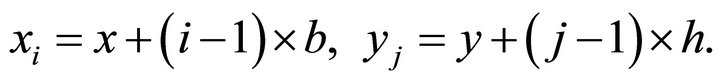
 . All sub-rectangles are defined with base(s)
  and height(s)
 . The start point
  of the sub-rectangle
  is then given by
 (7)
(7)
Consequently, the sub-rectangle  and its perimeter
  are written as
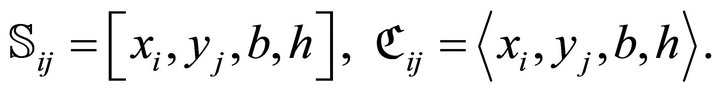 (8)
(8)
As discussed in [1] (Sections 3.4, 4), instead of the elements of a tridiagonal matrix, CCE can readily accept the coefficients of a complex polynomial, eventually of very high degree, with several roots of high multiplicity, as well as with closely spaced roots.
2. Parallelizing the Code
2.1. Theoretical Expectations
The main program of the code, so-called CCEDRIVER, examines if partitioning the given rectangle  is necessary and sets accordingly the logical variable PARTITION. In this case, CCEDRIVER proceeds with partitioning
  by calling an appropriate subroutine, socalled PARTITIONING. Furthermore, COUNTING is the subroutine which calculates by Equations (7) and (8) the perimeter
  of a sub-rectangle
 , calls repeatedly DCRKF54 to integrate along
 , and thus computes the number
  of the roots lying in
  (cf. Equation (6)); CNTALL is its driving subroutine which repeats the counting of the roots for all sub-rectangles. Next, ROOTFINDING is the subroutine which calls for a sub-rectangle
  the code that implements the cooperation of the double-precision and the multiple-precision NRs (so-called NR2; [1], Section 3.3), and thus computes the
  roots lying in
 ; RTSALL is its driving subroutine which repeats rootfinding for all sub-rectangles.
Algorithmically, the composed procedure has the following form.
PROGRAM CCEDRIVER
...
LOGICAL :: PARTITION
...
IF (PARTITION) THEN CALL PARTITIONING(...)
CALL CNTALL(...)
CALL RTSALL(...)
ELSE CALL COUNTING(...)
CALL ROOTFINDING(...)
END IF
...
END PROGRAM CCEDRIVER
:::
SUBROUTINE CNTALL(...)
...
DO I = 1, NMR DO J = 1, NMR CALL COUNTING(...)
END DO END DO
...
END SUBROUTINE CNTALL
:::
SUBROUTINE RTSALL(...)
...
DO I = 1, NMR DO J = 1, NMR CALL ROOTFINDING(...)
END DO END DO
...
END SUBROUTINE RTSALL
:::
where , three colons indicate omitted code outside a program unit, and three dots indicate omitted code inside a program unit.
Apparently, CCEDRIVER proceeds first with the counting of the roots by calling CNTALL or COUNTING (dependent on the value assigned to PARTITION) and second with the rootfinding by calling RTSALL or ROOTFINDING. Consequently, the execution inside CCEDRIVER proceeds in serial. This has not to be the case, however, inside CNTALL and RTSALL. Since counting the roots and rootfinding are processes repeated independently for each sub-rectangle , the corresponding subroutines can run in parallel on multi-core machines, with each available thread processing a part of the
  sub-rectangles.
Thus, theoretically, it is expected that the code can be efficiently parallelized inside the subroutines CNTALL and RTSALL with respect to the  sub-rectangles to be processed. Such theoretical expectations are carefully tested here by carrying out numerical experiments with random complex tridiagonal matrices and high-degree polynomials as well.
2.2. OpenMP Parallelization
The Open Multi-Processing (OpenMP; http//openmp.org/) is an Application Program Interface (API), jointly defined by a group of major computer hardware and software vendors, supporting shared-memory parallel programming in C/C++ and Fortran, for platforms ranging from desktops to supercomputers. Several compilers from various vendors or open source communities implement the OpenMP API. Among them, the GNU Compiler Collection (GCC; http://gcc.gnu.org/) includes a Fortran 95 compiler, so-called “gfortran” (http://gcc.gnu. org/fortran/), licensed under the GNU General Public License (GPL; http://www.gnu.org/licenses/gpl.html). The official manual of gfortran can be found at http://gcc. gnu.org/onlinedocs/gcc-4.7.0/gfortran.pdf. The GCC 4.7.x releases, including corresponding gfortran 4.7.x releases, support the OpenMP API Version 3.1. The official manual of this version can be found at http://www.openmp. org/mp-documents/OpenMP3.1.pdf. This OpenMP version is used here by gfortran.
To enable the processing of the OpenMP directive sentinel !$OMP, gfortran is invoked with the “-fopenmp” option. If so, then all lines beginning with the sentinels !$OMP and !$ are processed by gfortran.
To parallelize the subroutines CNTALL and RTSALL, we apply to them several OpenMP directives. Concerning CNTALL, for instance, we write the code
SUBROUTINE CNTALL(...)
...
!$OMP PARALLEL DEFAULT(...) PRIVATE(...) &
!$OMP& FIRSTPRIVATE(...) REDUCTION(...)
!$...
...
!$OMP DO SCHEDULE(...)
DO I = 1, NMR
!$...
...
DO J = 1, NMR
!$...
...
CALL COUNTING(...)
!$...
...
END DO
!$...
...
END DO
!$OMP END DO
!$OMP END PARALLEL
...
END SUBROUTINE CNTALL The sentinel !$ followed by three dots, !$..., denotes code (omitted here) to be compiled only when OpenMP is invoked. The PARALLEL and END PARALLEL directives define a parallel construct. The structured block of code enclosed in a parallel construct is executed in parallel by the machine’s available threads. The code placed directly in a parallel construct is its “lexical extend”, while, in turn, the lexical extend plus all the code called by it is the “dynamic extend” of the parallel construct; for instance, COUNTING and all code called by it lie in the dynamic extend of the parallel construct shown above. Several data-sharing attribute clauses can be linked to a PARALLEL directive, like DEFAULT, PRIVATE, FIRSTPRIVATE, REDUCTION, etc. Three parenthesized dots, next to their names, denote clauses linked to such directives; for instance, we mostly declare DEFAULT(SHARED), indicating that all variables in a parallel construct are to be shared among the available threads, except, eventually, for variables (or common blocks) named explicitly in a PRIVATE directive.
The DO and END DO directives define a loop worksharing construct, which distributes the loop computations over the available threads; so, each thread computes part of the required iterations. Several clauses are permitted to be linked to the DO directive, like SCHEDULE, PRIVATE, etc. Three parenthesized dots next to their names denote clauses linked to such directives. For instance, we write SCHEDULE (STATIC[,CHUNK]), indicating that all iterations are to be divided into pieces of size CHUNK and then to be statically assigned to the available threads (if CHUNK is not specified, then the iterations are evenly divided contiguously among the threads). On the other hand, the mostly used SCHEDULE(DYNAMIC[,CHUNK]) indicates that all iterations are to be divided into pieces of size CHUNK (if not present, then by default CHUNK = 1), and then to be dynamically assigned to the available threads, so that when a thread finishes one chunk, it is dynamically assigned another.
To parallelize the subroutine RTSALL, we follow a similar procedure. Parallel programming details are not analysed in this paper. We have mentioned only OpenMP directives that have been used in our code; certain significant issues, mainly concerning data environment, should be carefully taken into account by interested readers.
3. The Computations
3.1. Computational Environment and Software Used
Our computer comprises an Intel® CoreTM i7-950 processor with four physical cores. This processor possesses the Intel Hyper-Threading Technology, which delivers two processing threads per physical core. gfortran has been installed in this computer by the TDM-GCC “Compiler Suite for Windows” (http://tdm-gcc.tdragon.net/), which is free software distributed under the terms of the GPL. To calculate  values of the Fortran intrinsic function SQRT, our computer needs
  in double precision (i.e. KIND = 8) and almost the same time in high precision (i.e. KIND = 10), and
  in the precision of 256 digits with the MPFUN90 System (available in http://crd-legacy.lbl.gov/~dhbailey/mpdist; licensed under the Berkeley Software Distribution License found in that site).
In the numerical experiments of this study, we use an efficient algorithm for computing the coefficients of the characteristic polynomial of a general square matrix [6], abbreviated to CPC as in [1] (Section 3). Thus, in all computations involving polynomials, CCE makes use of the time-saving Horner’s scheme. In [1] (Section 3.3), we have compared the eigenvalues computed by CCE with respective results of an efficient and very fast code, abbreviated to CXR ([1], Section 3), solving general complex polynomial equations ([7]; this Fortran code, named cmplx_roots_sg.f90, can be found in http://www.astrouw. edu.pl/~jskowron/cmplx_roots_sg/; it is licensed under the GNU Lesser GPL, Version 2 or later, or under the Apache License, Version 2; details on these licences are given in the documents “LICENSE” and “NOTICE”, found in the same site). The CPC algorithm, as well as the subroutine CMPLX_ROOTS_GEN with its subsidiaries CMPLX_LAGUERRE, CMPLX_LAGUERRE2 NEWTON, and SOLVE_Quadratic_EQ (these four contained in cmplx_roots_sg.f90), have been modified so that to work in MPFUN90’s multiprecision.
The task of the present study is to compare execution times when CCE runs in serial and in parallel (the accuracy of CCE has been tested and verified in [1]). This task is accomplished by performing several numerical experiments with random complex tridiagonal matrices, and random complex high-degree polynomials as well.
3.2. Numerical Experiments and Comparisons
First, we perform numerical experiments with random complex tridiagonal matrices, constructed in the MPFUN 90’s multiprecision environment, as described in [1] (Section 3.3). We study tridiagonal matrices of order n = 128, 256, 400, and 512. In this work, the region  is assumed to be the “primary rectangle”
 ![]() ([1], Section 3.3),
([1], Section 3.3),  , containing all n roots, eventually determined by the numerical results of the CXR code. In all cases examined, the primary rectangle
 ![]() is partitioned into
is partitioned into  sub-rectangles.
Table 1 shows execution times for CPC, CXR, CNTALL-Serial, RTSALL-Serial, CCE-Serial, CNTALLParallel(S), RTSALL-Parallel(S), CCE-Parallel(S), CNTALL-Parallel(D), RTSALL-Parallel(D), and CCE-Parallel(D). In these names, the label “Serial” denotes execution times when CCE runs in serial; the label “Parallel(S)” denotes execution times when CCE runs in parallel under the loop-construct directive SCHEDULE(STATIC); and the label “Parallel(D)” denotes execution times when CCE runs in parallel under the loop-construct directive SCHEDULE(DYNAMIC).
To compare results of Table 1, called “present”, with corresponding results of [1] (Table 2), called in turn “previous”, we link: 1) the “present” group labeled “CNTALL-Serial” with the “previous” column labeled “DCRKF54(P)”, and 2) the “present” group labeled “RTSALL-Serial” with the “previous” column labeled “NR2 (P)”. We remark that the “present” times spent on counting the roots are greater than the “previous” ones for the cases n = 128, 256, and 400, since now P is partitioned into 16,384 sub-rectangles; while, for instance, in the “previous” case n = 128, P is partitioned into just 144 sub-rectangles.
On the other hand, the “present” time spent on counting the roots for the case n = 512 becomes less than the “previous” one. Apparently, counting the roots on much more sub-rectangles turns to be time-saving for large n, since the perimeters of the 16,384 sub-rectangles, along which the integral (1) is now computed, decrease dramatically in length; accordingly, the “present” times
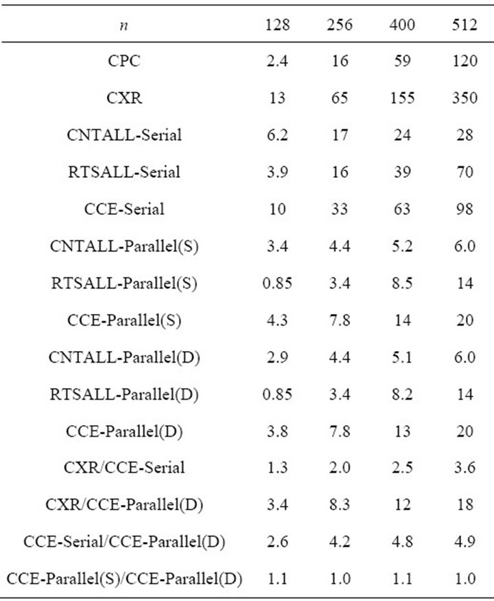
Table 1. Execution times for the codes appearing in the left column, and corresponding time ratios, in numerical experiments with random complex tridiagonal matrices constructed as in [1] (Section 3.3); n is the order of the tridiagonal matrix. Times less than 1 s are rounded to two decimal digits; times next to 1 s and less than 10 s are rounded to one decimal digit; times next to 10 s and less than 100 s are rounded to the nearest integer; times next to 100 s are rounded to the nearest zero or five.
spent on such computations become less than the “previous” ones. Furthermore, working with much more subrectangles turns to be in favour of computing the roots, since, now, each sub-rectangle contains a significantly less number of roots to be computed, and feeding the Newton-Raphson code with random guesses ([1], Section 3.2) is proved to be highly efficient. Thus all “present” times spent on computing the roots are less than the “previous” ones. Likewise, the “present” total execution times become less than the “previous” ones for the cases .
.
Next, the time ratio CCE-Serial/CCE-Parallel(D) seems to be significant for checking the degree that theoretical expectations are fulfilled in the implementation of OpenMP parallelization on multi-core machines. In particular, since this time ratio takes values larger than 4 and up to ~5 (with the exception of the case n = 128), it becomes apparent that there is an almost equal sharing of the computational volume among the 4 cores available in the processor of our computer. Apparently, the additional gain is due to the hyper-threading technology possessed by this processor.
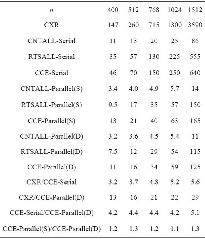
Table 2. Execution times for the codes appearing in the left column, and corresponding time ratios, in numerical experiments with random complex polynomials constructed under prescriptions similar to those of [1] (Section 3.3); n is the degree of the polynomial. Times less than 1 s are rounded to two decimal digits; times next to 1 s and less than 10 s are rounded to one decimal digit; times next to 10 s and less than 100 s are rounded to the nearest integer; times next to 100 s are rounded to the nearest zero or five.
Comparing execution times for Parallel(S) and Parallel(D) processing, we find that the corresponding values deviate slightly each other, i.e. the corresponding time ratio deviates slightly from unity. It is worth remarking, however, that in all cases examined the (even small) gain is on the side of Parallel(D); in simple words, it seems better to leave the machine to decide how to share the computational work.
Second, we accomplish numerical experiments with random complex polynomials of degree n = 400, 512, 768, 1024, and 1512. They are constructed in the MPFUN90’s multiprecision environment as described in [1], with the clarification that the n successively derived random complex numbers  are assigned to the corresponding polynomial coefficients of the degree-n polynomial
 ,
, ; while, as usual, the
  - th coefficient is assigned the value
 .
.
Concerning the results of Table 2, we arrive at conclusions similar to those above. We emphasize on the fact that CCE running in parallel is proved ~13 times faster than the CXR code in the case of a degree—400 complex polynomial, and increases gradually up to ~30 times faster than CXR in the case of a degree—1512 complex polynomial.
A Fortran package implementing the parallelized CCE code, called parcce.f95, is available on request to the first author (vgeroyan@upatras.gr); it is licensed under the GNU General Public License, Version 3 (GPLv3, http:// www.gnu.org/licenses/gpl-3.0.html). Note that the package parcce.f95 does not include the MPFUN90 System; interested readers can download MPFUN90 from the site given in Section 3.1. Note also that the CXR code, which has been used in the numerical experiments of this study for the purpose of comparing execution times, is not included in the package parcce.f95; readers interested in using CXR can download this code from the site given in Section 3.1.
4. Conclusion
In this study, we have pointed out that the CCE code presented in [1] can be parallelized. Our numerical experiments have shown that, for all cases examined, the parallelized CCE code took full advantage of the fourcore processor of our computer. It has been also verified that there was an additional gain due to the hyperthreading technology of this processor.
5. Acknowledgements
The authors acknowledge the use of: the Fortran-90 Multiprecision System (Refs. [4,5]); the algorithm for computing the coefficients of the characteristic polynomials of general square matrices (Ref. [6]), abbreviated to CPC in both [1] and the present study; and the general complex polynomial root solver (Ref. [7]), abbreviated to CXR in both [1] and the present study.
REFERENCES
- F. N. Valvi and V. S. Geroyannis, “Counting and Computing the Eigenvalues of a Complex Tridiagonal Matrix, Lying in a Given Region of the Complex Plane,” International Journal of Modern Physics C, Vol. 24, No. 2, 2013, Article ID: 1350008(1-10). doi:10.1142/S0129183113500083
- W. W. Chen, “Introduction to Complex Analysis,” 2008. http://rutherglen.science.mq.edu.au/wchen/lnicafolder/lnica.html
- V. S. Geroyannis and F. N. Valvi, “A Runge-KuttaFehlberg Code for the Complex Plane: Comparing with Similar Codes by Applying to Polytropic Models,” International Journal of Modern Physics C, Vol. 23, No. 5, 2012, Article ID: 1250038(1-15). doi:10.1142/S0129183112500386
- D. H. Bailey, “A Fortran 90-Based Multiprecision System,” ACM Transactions on Mathematical Software, Vol. 21, No. 4, 1995, pp. 379-387. doi:10.1145/212066.212075
- D. H. Bailey, “A Fortran-90 Based Multiprecision System,” RNR Technical Report, RNR-94-013, 1995, pp. 1- 10.
- S. Rombouts and K. Heyde, “An Accurate and Efficient Algorithm for the Computation of the Characteristic Polynomial of a General Square Matrix,” Journal of Computational Physics, Vol. 140, No. 2, 1998, pp. 453-458. doi:10.1006/jcph.1998.5909
- J. Skowron and A. Gould, “General Complex Polynomial Root Solver and Its Further Optimization for Binary Microlenses,” arXiv:1203.1034v1 [astro-ph.EP], 2012, pp. 1-29.