Applied Mathematics
Vol.4 No.3(2013), Article ID:28855,8 pages DOI:10.4236/am.2013.43070
Modeling of Surface Waves in a Fluid Saturated Poro-Elastic Medium under Initial Stress Using Time-Space Domain Higher Order Finite Difference Method
1Department of Applied Mathematics, Birla Institute of Technology, Ranchi, India
2Department of Mathematics, RVS College of Engineering & Technology, Jamshedpur, India
Email: anjana_pghorai@yahoo.co.in, rekha.tiwari68@gmail.com
Received December 26, 2012; revised February 5, 2013; accepted February 13, 2013
Keywords: Love Waves; Fluid Saturated Initially Stressed Porous Layer; Time-Space Domain; Finite Difference Scheme; Accuracy; Dispersion Analysis; Phase Velocity
ABSTRACT
In this present context, mathematical modeling of the propagation of surface waves in a fluid saturated poro-elastic medium under the influence of initial stress has been considered using time dependent higher order finite difference method (FDM). We have proved that the accuracy of this finite-difference scheme is 2M when we use 2nd order time domain finite-difference and 2M-th order space domain finite-difference. It also has been shown that the dispersion curves of Love waves are less dispersed for higher order FDM than of lower order FDM. The effect of initial stress, porosity and anisotropy of the layer in the propagation of Love waves has been studied here. The numerical results have been shown graphically. As a particular case, the phase velocity in a non porous elastic solid layer derived in this paper is in perfect agreement with that of Liu et al. (2009).
1. Introduction
The simulation of surface waves propagating in a fluid saturated poro-elastic media is of great importance to seismologists due to its possible applications in geophysical prospecting, reservoir engineering and survey techniques for understanding the cause and estimation of damage due to natural and manmade hazards. Also the difficulty in exploring natural resources is gradually increasing as the nature of the reservoir is more complex and heterogeneous than it was assumed in past and the characterization of the subsurface materials as fluid saturated porous media is more realistic. It is also more accurate to consider soil as two phase composite materials, granular solid and pore fluid. The size of pores is assumed to be small and macroscopically speaking, their average distribution is uniform.
Since poro-elastic theory was developed by Biot [1-3] many efforts have been made in using experimental and numerical methods to characterize elastic wave propagation in porous, liquid-saturated solids. Quite a good amount of information about the effect of initial stress on propagation of surface waves is available in the literature of many authors namely, A. M. Abd-Alla [4], S. Gupta
[5], Shishir Gupta [6]. In these papers they have followed the conventional analytical method to solve these problems. But recently the finite difference method appears as an important tool for numerical simulations of partial differential equations and has been used widely in simulating elastic waves. Due to easy and straightforward approach, robustness, requiring small memory and computation time, the Finite Difference Methods are the most popular methods for seismic modeling. Also wave equation modeling in the time domain is popular because of its easy implementation and accuracy, compared to frequency domain modeling. In time-domain modeling, higher-order differencing operators are used to reduce the required spatial sampling. Virieux [7,8] have used velocity-stress finite difference method for the propagation of P-SV wave and SH wave in heterogeneous media. To improve the accuracy and stability of finite difference scheme, many authors have used and developed different types of difference schemes. Levander [9] applied 4th order approximation in space to the P-SV scheme. Hayashi and burns [10] developed finite difference scheme with variable grids. R. W. Graves [11] discussed the simulation of seismic wave propagation in 3D elastic media using staggered-grid finite difference method. Kristek et al. [12] considered seismic wave propagation in viscoelastic media using 3D forth order staggeredgrid finite difference scheme. Saenger et al. [13] have considered the rotated staggered grid finite difference method. Bohlen et al. [14] discussed the accuracy of heterogeneous staggered-grid finite-difference modeling. Kristek et al. [15] discussed on the accuracy of the finite-difference schemes for the one dimensional elastic problem. Tessmer [16] discussed Seismic finite difference modeling with spatially variable time steps. Finkelstein et al. [17] developed finite difference time domain dispersion reduction schemes. Y. Liu et al. [18,19] discussed advanced and truncated finite difference method for seismic modeling and Y. Liu et al. [20] employed a plane wave theory and the Taylor series expansion of dispersion relation to derive the FD coefficients in the joint time-space domain for the scalar wave equation with second-order spatial derivatives. They demonstrated that the method has greater accuracy and better stability than the conventional method. Dublain [21] has demonstrated the advantages of the higher order difference scheme. Lie et al. [22] designed spatial finite difference stencils on a time-space domain to simulate wave propagation in acoustic vertically transversely isotropic medium. Two-dimensional dispersion analysis and numerical modeling demonstrate that this stencil has greater precision than one used in a conventional F. D. Lie et al. [23] discussed finite difference numerical modeling in two phase anisotropic media with even order accuracy. Zhu et al. [24] developed finite difference modeling of the seismic response of fluid saturated, porous, elastic solid using Biot theory. Lie et al. [25] developed a time-space domain dispersion-relationbased staggered-grid finite-difference schemes for modeling the scalar wave equation. Also, the new stencils can adopt a larger time step. Dispersion analysis and numerical modeling results demonstrate that the new stencils have greater accuracy and can effectively suppress the dispersion and retain the waveform.
In this paper, following [22,25] we have modeled the Love waves in a fluid saturated poro-elastic media under the influence of initial stress using time-space domain higher order finite difference method. The dispersion equation has been obtained and the presence of the porosity parameter, the non-dimensional anisotropic parameter and the non-dimensional parameters due to the initial stress in the equation of dispersion shows the significant effect on the propagation of love waves. The phase velocity of Love wave has been computed numerically and presented graphically. It is observed that the anisotropic parameter in the porous layer and the porosity of the layer both have the increasing effect but the initial stress field has an decreasing effect on the phase velocity of Love wave.
2. Formulation of the Problem and Its Finite Difference Approximation
2.1. Formulation
We consider a model consisting of fluid saturated anisotropic poro-elastic layer of finite thickness under compressive initial stress; the x-axis is chosen parallel to the layer in the direction of propagation of surface wave and the z-axis is taken vertically downward.
Neglecting the viscosity of the fluid and the body force, Biot’s dynamical equations for the fluid-saturated anisotropic porous layer under compressive initial stress are given by [1,2]
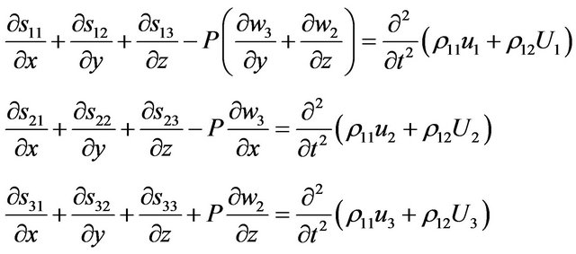
(1)
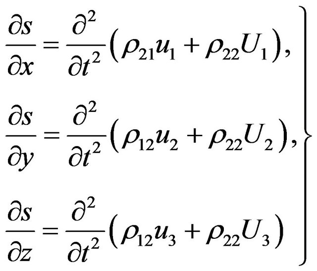 (2)
(2)
where , the initial stress along x axis,
  , are the components of stress tensor in the solid skeleton,
  is the reduced pressure of the fluid (
 is the pressure in the fluid, and
  is the porosity of the porous layer),
  are the components of the displacement vector of the solid and
  are those of fluid of the porous aggregate,
  are the angular displacement vectors. The dynamic coefficients,
  take into account of the inertia effects of the moving fluid and are related to the densities of the solid
  the fluid
  and the layer
  by the equation
 ,
,  so that the mass density of the aggregate is
 .
.
Also the dynamic coefficients, moreover, obey the inequalities 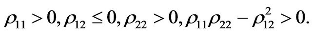
The stress-strain relations for the fluid-saturated anisotropic porous layer under initial stress are given by
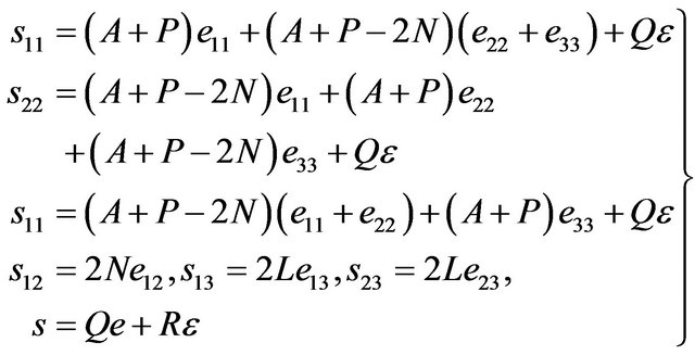 (3)
(3)
where  and
and  and
and 
are the corresponding dilatations which opposite in sign, A, N, L correspond to the familiar Lame’s constants, R is the amount of pressure required on the fluid to force a certain volume of the fluid into the aggregate while the total volume remains constants and Q is the coefficient of coupling between the volume change of the solid and that of the fluid.
Also the angular displacements are given by
 and
and 
For the propagation of Love waves along x axis, using conventional conditionsi.e.  and
and 
where  and
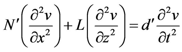
and  the equations of motion given by (1) and (2) are reduced to the form
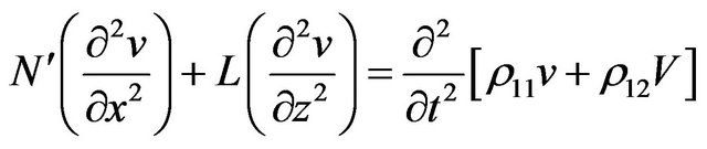 (4)
(4)
 (5)
(5)
where and
and  is the non-dimensional parameters due to the initial stress.
Eliminating the component of liquid displacement V from (4) and (5) we have
 (6)
(6)
where
 (7)
(7)
From the Equation (6) it can be seen that the velocities of shear waves in the porous medium in x and z directions are  and
and  respectively and from (7),
  is less than
 and hence, in turn, less than
 , the density of the elastic layer for all values of
 . This shows that the velocities of shear waves in x and z directions in the fluid saturated porous layer will be more those of corresponding elastic layer.
2.2. Finite Difference Approximation
Equation (6) can be written as
 (8)
(8)
where  and
and , the velocity of shear wave in the porous medium in x direction.
The shear wave velocity in the x-direction may be expressed as
 (9)
(9)
where  and
and , the velocity of the shear wave in the corresponding non-porous, initial stress free anisotropic elastic medium along the direction of x. Also,
 (10)
(10)
are the non-dimensional parameters for the material of the porous layer [1,2].
To improve the accuracy we have considered here the higher order finite difference scheme for spatial derivatives as
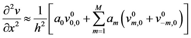 (11)
(11)
 (12)
(12)
As generally higher order finite difference on temporal derivatives scheme requires large space in the computer memory and usually unstable, 2nd order finite difference scheme is used for temporal derivatives as
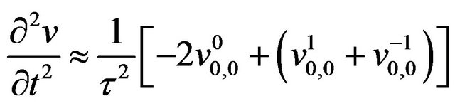 (13)
(13)
where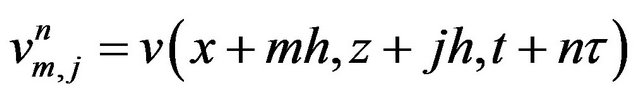 ,
,  is the grid size and
  is the time step.
Using (11)-(13) into (8) we have
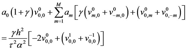
(14)
Using the plane wave theory, let us consider
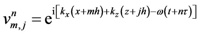 (15)
(15)
Substituting (15) into (14) and simplifying, we have
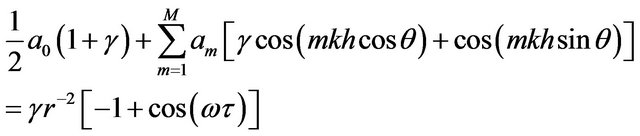
(16)
where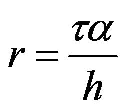 ,
,  ,
,  , being the propagation direction angle of the plane wave.
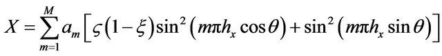
Using the Taylor series expansion for cosine functions, we have from (16)
(17)
Comparing the coefficients of , we get,
 (18)
(18)
 , (19)
where 
This equation indicates that the coefficients  are the function of
  . To obtain a single set of coefficients, an optimal angle has to be chosen. We solve the equation (19) to get
  by using
  and then
  can be obtained from (18).
3. Errors and Accuracy
The error function of Equation (17) can be written as
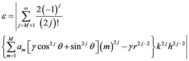
(20)
Since the minimum power of h in the error function (20) is 2M, the accuracy of this finite difference scheme is 2M when we use 2nd order time domain finite difference scheme and 2M-th order space domain finite difference scheme. The increase in M may decrease the magnitude in errors but may not increase the order of accuracy. As we have used the finite difference scheme in both time domain and space domain, the wave Equation (8) can be solved in both time domain and space domain simultaneously by (14).
4. Dispersion Analysis
Let us define a parameter  to describe the dispersion of Finite difference by using Equation (17) as follows:
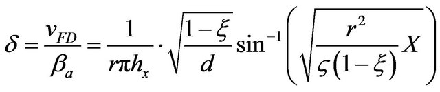 (21)
(21)
where
(22)
If  is equal to 1, then there is no dispersion. However, if
  is far from 1, a large dispersion will occur. In calculating
 ,
, , the grid points per wavelength, ranges from 0.04 to 0.5 and the variation of
  is from 0 to
 .
.
The presence of d, the porosity parameter, 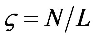 , the non-dimensional anisotropic parameter and
  , the non-dimensional parameters due to the initial stress shows that the dispersion curve are affected by these also.
It may be noted that  gives the fraction of porosity in the layer. If the layer is non-porous then
  and hence
  and we find
and  which leads to
  i.e.
i.e.
 .
.
Again if  then
then  and the layer becomes a fluid, and in that case the shear wave velocity in the layer cannot exist which so happens when
 .
.
Thus we have the following:
i) , when the layer is non-porous solid;
ii) , when the layer tends to be fluid;
iii) , when the layer is porous.
Here we study the dispersion curves for different grid points per wave length, velocities, porosity, anisotropic parameters, non-dimensional parameters due to the initial stress and time steps.
5. Numerical Calculation and Discussions
The numerical calculation of the Equation (21) has been done for different values of the parameters g, d and by taking, . The phase velocity
  of Love wave from the Equation (21) versus
 , the grid points per wavelength, has been computed for different values of
 ,
,
 ,
,  the propagation angle
 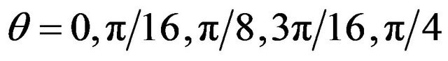 and
and .
.
Figures 1-3 display the dispersion curves of Love waves with respect to different grid points per wave length, at different values of M in a homogeneous non porous initial stress free elastic solid, porous isotropic and anisotropic layer under the influence of initial stress respectively. It is found that dispersion is more for the lower values of M and less for higher values of M. Here
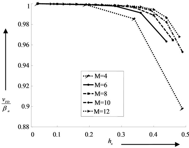
Figure 1. Dispersion curves for love waves for different values of M when ,
,  and
and .
.
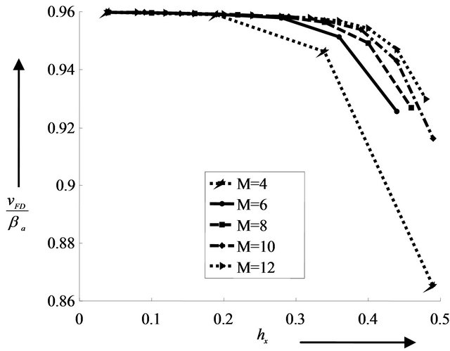
Figure 2. Dispersion curves for love waves for different values of M when ,
,  and
and .
.
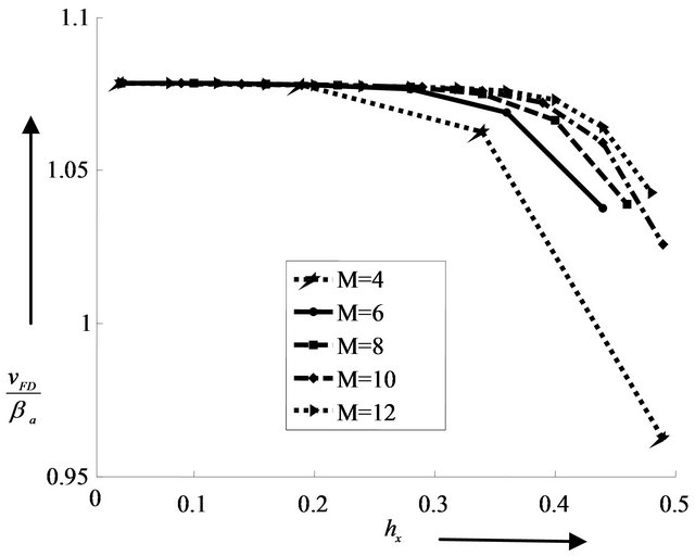
Figure 3. Dispersion curves for love waves for different values of M when ,
,  and
and .
.
also it is observed that the increase in porosity and anisotropy leads to the increase in the magnitude of the phase velocity of Love waves whereas the increase in initial stress parameter leads to decrease in the phase velocity of Love waves.
Figure 4 shows the effect of porosity in the dispersion of phase velocity of Love waves with respect to different grid points per wave length in a homogeneous, isotropic porous layer without initial stress field and under the influence of initial stress. It is observed that as the porosity increases, that is, as the value of d decreases, the phase velocity of Love wave increases and decreases as the initial stress field increases.
Figures 5 and 6 show the effect of initial stress field in the propagation of Love waves with respect to different grid points per wave length in a isotropic and an-isotropic non-porous elastic solid and fluid saturated porous layer. As the anisotropy increases, the phase velocity of Love wave increases and the phase velocity of Love
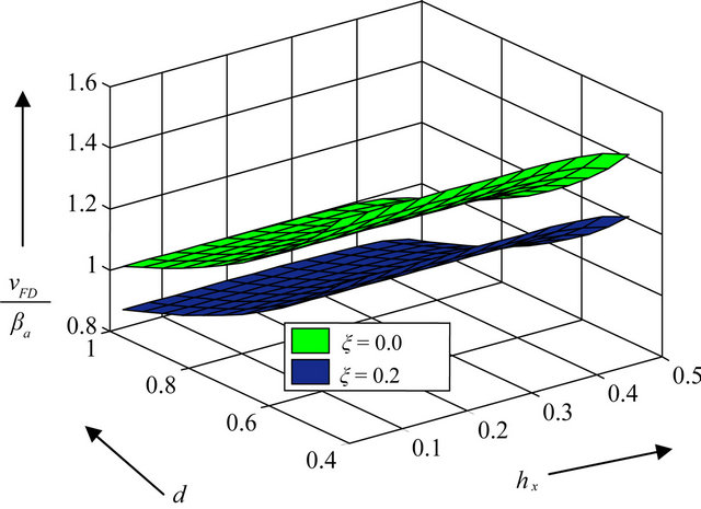
Figure 4. Dispersion curves for love waves for different values of porosity and initial stress
  when
when .
.
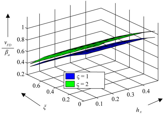
Figure 5. Dispersion curves for love waves for different values of initial stress ξ and anisotropic parameter  when d = 1.
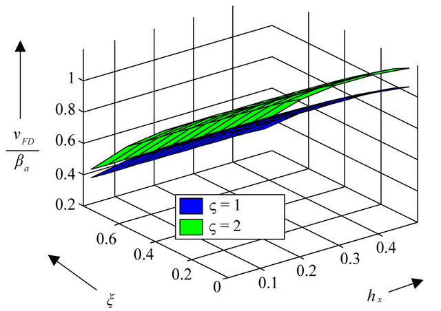
Figure 6. Dispersion curves for love waves for different values of initial stress  and anisotropic parameter
  when
when .
.
wave decreases as the initial stress field increases.
Figures 7 and 8 display the dispersion curves of Love waves with respect to different grid points per wave length at different angles of propagation in a homogeneous fluid saturated porous layer and non-porous elastic solid layer for different values of initial stress respectively. It is observed that dispersion is more for the lower degree of propagation angles as compare to the higher degree of angle. Phase velocity is more in fluid saturated porous layer than in non-porous elastic solid layer. Later is the case discussed by Yang Liu et al. [20].
Figures 9 and 10 displays the dispersion curves of Love waves with respect to different grid points per wave length at different time steps in a homogeneous non porous elastic solid and non-homogeneous, anisotropic fluid saturated porous layer without initial stress field and under the influence of initial stress respectively. It is found that initially the dispersion is less and as time increases, the dispersion increases.
6. Conclusion
It is observed that the higher order time dependent finite difference method plays an important role in the propagation of Love waves in a porous layer under the influence of initial stress. Graphically we have shown that the dispersion curves of Love waves are less dispersed for higher order finite difference method. It has also been shown that initially the dispersion is less and as time increases, the dispersion increases. The significant effect of porosity, anisotropy and initial stress simultaneously in the propagation of Love waves in a porous layer has also been discussed. The phase velocity of Love wave is more in fluid saturated porous layer than in non-porous elastic solid layer. The anisotropy has an increasing effect whereas the initial stress field has a decreasing effect on the
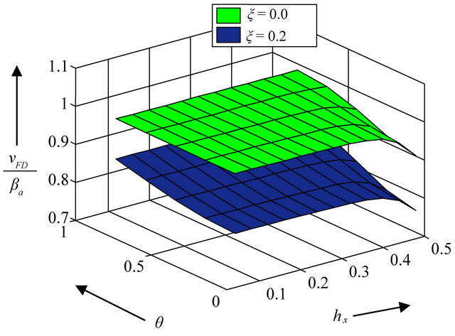
Figure 7. Dispersion curves for love waves at different propagation angle  for different values of initial stress
  when anisotropic parameter
  when
when .
.
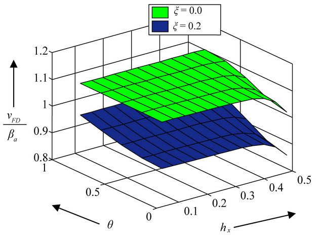
Figure 8. Dispersion curves for love waves at different propagation angle  for different values of initial stress
  when anisotropic parameter
  when
when .
.
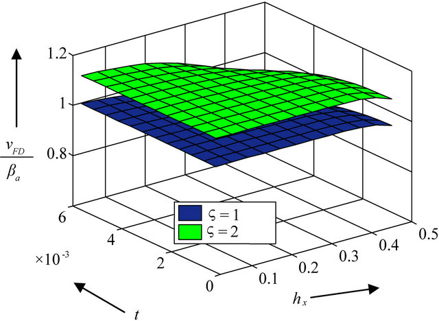
Figure 9. Dispersion curves for love waves waves at different time steps for different values of anisotropic parameter  when initial stress
  and
and .
.
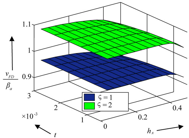
Figure 10. Dispersion curves for love waves waves at different time steps for different values of anisotropic parameter  when initial stress
  and d = 0.8.
phase velocity of Love waves.
REFERENCES
- M. A. Biot, “Theory of Propagation of Elastic Solid in a Fluid-Saturated Porous Solid 1. Low-Frequence Range,” Journal of the Acoustical Society of America, Vol. 28, 1956, pp. 168-178. doi:10.1121/1.1908239
- M. A. Biot, “Theory of Propagation of Elastic Solid in a Fluid-Saturated Porous Solid II. Low-Frequence Range,” Journal of the Acoustical Society of America, Vol. 28, 1956, pp. 179-191. doi:10.1121/1.1908241
- M. A. Biot, “Surface Instability in Finite Anisotropic Elasticity under Initial Stress,” Proceedings of the Royal Society A, Vol. 273, No. 1354, 1963, pp. 329-339. doi:10.1098/rspa.1963.0092
- A. M. Abd-Alla, S. R. Mahmoud and M. I. R. Helmi, “Effect of Initial Stress and Magnetic Field on Propagation of Shear Wave in Non-Homogeneous Anisotropic Medium under Gravity Field,” The Open Applied Mathematics Journal, Vol. 3, No. 1, 2009, pp. 58-65. doi:10.2174/1874114200903010058
- S. Gupta, A. Chattopadhyay and D. K. Majhi, “Effect of Initial Stress on Propagation of Love Waves in an Anisotropic Porous Layer,” Journal of Solid Mechanics, Vol. 2, No.1, 2010, pp. 50-62.
- S. Gupta, A. Chattopadhyay, S. K. Vishwakarma and D. K. Majhi, “Influence of Rigid Boundary and Initial Stress on the Propagation of Love Wave,” Applied Mathematics, Vol. 2, No. 5, 2011, pp. 586-594. doi:10.4236/am.2011.25078
- J. Virieux, “SH-Wave Propagation in Heterogeneous Media: Velocity Stress Finite Difference Method,” Geophysics, Vol. 49, No. 11, 1984, pp. 1933-1957. doi:10.1190/1.1441605
- J. Virieux, “P-SV Wave Propagation in Heterogeneous Media: Velocity Stress Finite Difference Method,” Geophysics, Vol. 51, No. 4, 1986, pp. 889-901. doi:10.1190/1.1442147
- A. Levander, “Fourth-Order Finite Difference P-SV Seismograms,” Geophysics, Vol. 53, No. 11, 1998, pp. 1425- 1436. doi:10.1190/1.1442422
- K. Hayashi and D. R. Burns, “Variable Grid Finite-Difference Modeling Including Surface Topography,” 69th Annual International Meeting, SEG, Expanded Abstracts, Vol. 18, 1999, pp. 523-527.
- R. W. Graves, “Simulating of Seismic Wave Propagation in 3D Elastic Media Using Staggered-Grid Finite Differences,” Bulletin of the Seismological Society of America, Vol. 86, No. 4, 1996, pp. 1091-1106.
- J. Kristek and P. Moczo, “Seismic Wave Propagation in Visco-Elastic Media with Material Discontinuities: A 3D Forth-Order Staggered-Grid Finite Difference Modeling,” Bulletin of the Seismological Society of America, Vol. 93, No. 5, 2003, pp. 2273-2280. doi:10.1785/0120030023
- E. H. Saenger and T. Bohlen, “Finite Difference Modeling of Viscoelastic and Anisotropic Wave Propagation Using the Rotated Staggered Grid,” Geophysics, Vol. 69, No. 2, 2004, pp. 583-591. doi:10.1190/1.1707078
- T. Bohlen and E. H. Saenger, “Accuracy of Heterogeneous Staggered-Grid Finite-Difference Modeling of Rayleigh Waves,” Geophysics, Vol. 71, No. 4, 2006, pp. T109- T115. doi:10.1190/1.2213051
- J. Kristek and P. Moczo, “On the Accuracy of the Finite-Difference Schemes: The 1D Elastic Problem,” Bulletin of the Seismological Society of America, Vol. 96, No. 6, 2006, pp. 2398-2414. doi:10.1785/0120060031
- E. Tessmer, “Seismic Finite Difference Modeling with Spatially Variable Time Steps,” Geophysics, Vol. 65, No. 4, 2000, pp. 1290-1293. doi:10.1190/1.1444820
- B. Finkelstein and R. Kastner, “Finite Difference Time Domain Dispersion Reduction Schemes,” Journal of Computational Physics, Vol. 221, No. 1, 2007, pp. 422-438. doi:10.1016/j.jcp.2006.06.016
- Y. Liu and M. K. Sen, “Advanced Finite-Difference Method for Seismic Modeling,” Geohorizons, Vol. 14, No. 2, 2009, pp. 5-16.
- Y. Liu and M. K. Sen, “A Practical Implicit Finite Difference Method: Examples from Seismic Modeling,” Journal of Geophysics and Engineering, Vol. 6, No. 3, 2009, pp. 231-249. doi:10.1088/1742-2132/6/3/003
- Y. Liu and M. K. Sen, “A New Time-Space Domain High-Order Finite Difference Method for the Acoustic Wave Equation,” Journal of Computational Physics, Vol. 228, No. 23, 2009, pp. 8779-8806. doi:10.1016/j.jcp.2009.08.027
- M. A. Dublain, “The Application of High-Order Differencing to the Scalar Wave Equation,” Geophysics, Vol. 51, No. 1, 1986, pp. 54-66. doi:10.1190/1.1442040
- Y. Liu and M. K. Sen, “Acoustic VTI Modeling with a Time-Space Domain Dispersion-Relation-Based FiniteDifference Scheme,” Geophysics, Vol. 75, No. 3, 2010, pp. A11-A17. doi:10.1190/1.3374477
- Y. Liu and W. Xiucheng, “Finite Difference Numerical Modeling with Even Order Accuracy in Two Phase Anisotropic Media,” Applied Geophysics, Vol. 5, No. 2, 2008, pp. 107-114. doi:10.1007/s11770-008-0014-6
- X. Zhu and G. A. McMechan, “Finite difference Modeling of the Seismic Response of fluid Saturated, Porous, Elastic Solid Using Biot Theory,” Geophysics, Vol. 56, No. 4, 1991, pp. 424-435.
- Y. Liu and M. K. Sen, “Scalar Wave Equation Modeling with Time-Space Domain Dispersion-Relation-Based Staggered-Grid Finite-Difference Schemes,” Bulletin of the Seismological Society of America, Vol. 101, No. 1, 2011, pp. 141-159. doi:10.1785/0120100041